Important Note on this material
These notes are heavily based on the following books/references. All the text and images that appear in these notes are not to be redistributed or shared in any way.
- CLRS = Introduction to Algorithms (3rd edition), T. Cormen, C. Leiserson, R. Rivest, and C Stein, 2009.
- DPV = Algorithms, S. Dasgupta, C. Papadimitriou, U. Vazirani, 2006.
- Algorithms, J. Erickson, 2013.
- Algorithm Design, J. Kleinberg and E. Tardos, 2005.
Final note: All possible mistakes and inconsistencies are mine (EZ) and I would be grateful if you report them immediately.
Syllabus
Exams
The following general rules apply to exams:
- All exams in this course are written tests and to be taken in classroom.
- Exams are *closed* books and notes, but you can have a cheatsheet with you, letter-size, one-side handwritten, no copies.
- Collaboration of any kind in exams is strictly prohibited.
- Students can use simple calculators, if needed.
Schedule and Topics
Note: The schedule may change at the discretion of the instructor.
Welcome to CSC 282/482
Lecture 01.18

Instructor
- Name: Eustrat Zhupa
- Residence: Apt. 2107 Wegmans Hall
- Email: ezhupa@cs.rochester.edu
Note: Please include "CSC282: ..." in the subject of your 'letter'.
Administrivia (1)
Course
- Title: Design and Analysis of Efficient Algorithms
- Time: Tue/Thu 9:40 - 10:55 (AM)
- Modality: In classroom.
Administrivia (2)
Components of the course are as follows:
- Lectures ($2 \times 1.25$ hours) + practice quizzes
- Recitation sessions
- Homework
- Exams
Administrivia (3)
Your grade is determined as follows:
- The two midterms are worth 20% each.
- Homework is worth 15%.
- Attendance is worth 5%.
- The final exam is worth 40%.
Students with Accommodations
Students of all backgrounds and abilities are welcome in this course.
- Reach out to the instructor to inform about your specific needs.
- For any other need reach out to the instructor to make the appropriate arrangements.
Readings

Readings relevant to the course include:
- Lecture materials
- Additional problems posted on BB
- Textbooks (see syllabus for more)
- [CLRS] = Introduction to Algorithms (3rd edition), T. Cormen, C. Leiserson, R. Rivest, and C Stein,2009
- [DPV] = Algorithms, S. Dasgupta, C. Papadimitriou, U. Vazirani, 2006
- Additional readings for specific topics.
Getting Help

There are several support options you can take advantage of:
- Instructor's office hours (see BB). Please let me know in advance.
- Teaching Assistants
- Problem Sessions (see schedule).
Topics (1)
In Design and Analysis of Efficient Algorithms the following concepts will be discussed:
- Greedy Algorithms and Dynamic Programming
- Solving classical problems with DP and Greedy Techniques
- Comparison between the two
- Analysis of the proposed solutions
Topics (2)
In Design and Analysis of Efficient Algorithms the following concepts will be discussed:
- Algorithms based on Graphs
- Solving classical problems that can be modelled on graphs: shortest paths, minimum spanning trees, matching, flows, etc.
- Comparison between different algorithms
- Analysis of the proposed solutions
Topics (3)
In Design and Analysis of Efficient Algorithms the following concepts will be discussed:
- Linear Programming and NP problems
- Simplex Method
- Gauss-Jordan elimination method
- Divide and Conquer Algorithms
- Computational Geometry
- Reductions
- NP class and related concepts
- Guest Lecture (TBA)
Asymptotic Analysis Refresher
Definition of complexity classes using asymptotic notation:
- $f(n)=O(g(n)) \Leftrightarrow (\exists c)~ (\forall n)~ f(n) \leq cg(n)$
- $f(n)=\Omega(g(n)) \Leftrightarrow g(n)=O(f(n))$
- $f(n)=\Theta(g(n)) \Leftrightarrow f(n)=O(g(n)) \land g(n)=O(f(n))$
Practice break

Have a great semester!
See you next time.
😎
Welcome to CSC 282/482
Lecture 2

Reminder: HW posted
Rod Cutting (1)
URod Enterprise buys long steel rods and cuts them into shorter pieces to sell. The management of URod Enterprise would like to know the optimal length for the cuts.
The problem is defined as follows:
- A (whole) rod of length $n$ inches can be cut in different ways (for free).
- A selling price $p_i$ in dollars ($i = 1, 2, \ldots, n$).
- Goal: Determine the maximum revenue $r_n$ obtainable by cutting up the rod and selling the pieces.
| Length $i$ | 1 | 2 | 3 | 4 | 5 | 6 | 7 | 8 | 9 | 10 |
| Price $p_i$ | 1 | 5 | 8 | 9 | 10 | 17 | 17 | 20 | 24 | 30 |
Rod Cutting (2)
The following procedure implements the naive recursive top-down approach. \begin{equation*} %\setlength\arraycolsep{1.5pt} \begin{array}{@{\quad}l} CutMaster(p, n) \\ \quad if ~ n==0 \\ \qquad return~ 0 \\ \quad q = -\infty \\ \quad for~ i=1 ~to~ n \\ \qquad q=max(q,p[i] + CutMaster(p,n-i)) \\ \quad return~ q \\ \end{array} \end{equation*}
[Run]
Quiz break

Dynamic Programming
Idea: Solve subproblems only once.
Subidea: Trade some memory for time.
There are two equivalent ways to implement a dynamic-programming approach:
- top-down with memoization: we write the procedure recursively in a natural manner, but save the result of each subproblem
- bottom-up method: sort the subproblems by size and solve them in size order, smallest first.
Rod Cutting (3)
The bottom-up version is even simpler: \begin{equation*} %\setlength\arraycolsep{1.5pt} \begin{array}{@{\quad}l} BottomUpCutMaster(p, n) \\ \quad \text{initialize r[0..n] as new array} \\ \quad r[0]=0 \quad//\quad \text{ no pain, no gain}\\ \quad for~ j=1~ to~ n \\ \qquad q = -\infty \\ \qquad for~ i=1 ~to~ j \\ \qquad\quad q=max(q,p[i] + r[j-i]) \\ \qquad r[j] = q \\ \quad return~r[n] \end{array} \end{equation*}
Thank you for the attention
See you next time
Welcome to CSC 282/482
Lecture 3
Reminder: HW1 posted
Memento
Where to cut?
In the rod cutting problem we try all possible cuts for computing the optimal solution.

Memento
Where to cut?
In the rod cutting problem we try all possible cuts for computing the optimal solution.


Coin Change Problem

| Input: |
|
| Output: |
|
Coin Change Problem (DP)
\begin{equation*} %\setlength\arraycolsep{1.5pt} \begin{array}{@{\quad}l} MakeChange(V, D) \\ \quad c[0] = 0 \\ \quad for~\nu = 1~to~V \\ \qquad min = \infty \\ \qquad i = n \\ \qquad while(i>0~and~D[i] <= \nu) \\ \qquad \qquad if~c[\nu - D[i]] < min \\ \qquad \qquad \qquad min = c[\nu - D[i]] \\ \qquad \qquad i = i - 1 \\ \qquad c[\nu] = min + 1 \\ \quad return~c[V] \\ \end{array} \end{equation*}
'Fat Oracle' approach
In order for a problem to admit a greedy algorithm, it must satisfy two properties:
- Optimal Substructure: an optimal solution of an instance of the problem contains within itself an optimal solution to a smaller subproblem (or subproblems).
- Greedy-choice Property:There is always an optimal solution that makes a greedy choice.

Quiz 3 break

5 minutes
Welcome to CSC 282/482
Lecture 4

The Report Mission
A draft report has five chapters. The report must be 600 pages long.
Goal: Edit the report so that the overall importance is maximized.
\begin{equation*} %\setlength\arraycolsep{1.5pt} \begin{array}{c@{\quad} c c c c } Chapter & Pages & Importance & \frac{I}{W} & \frac{W}{I} \\ 1 & 120 & 5 & 0.041 & 24 \\ 2 & 150 & 5 & 0.033 & 30 \\ 3 & 200 & 4 & 0.020 & 50\\ 4 & 150 & 8 & 0.053 & 18.75 \\ 5 & 140 & 3 & 0.021 & 46.6 \\ \end{array} \end{equation*}Knapsack Problems
Given $n$ objects and a knapsack (bag) capacity $C$, where object $i$ has weight $w_i$ and earns profit $p_i$, find values of $x_i$ to maximize the total profit: \begin{equation*} %\setlength\arraycolsep{1.5pt} \begin{array}{c} \sum_{i=1}^n x_i p_i \end{array} \end{equation*} Subject to \begin{equation*} %\setlength\arraycolsep{1.5pt} \begin{array}{c} \sum_{i=1}^n x_i w_i \leq C, 0\leq x_i \leq 1. \end{array} \end{equation*}
This problem is known as the fractional knapsack problem.
'Fat Oracle' Algorithm for Report Mission
\begin{equation*} %\setlength\arraycolsep{1.5pt} \begin{array}{@{\quad}l} ContKnapsack(a, C) \\ \quad sort~a \quad \text{ // array sorted by ratio } \\ \quad weight=0 \\ \quad i=1 \\ \quad while(i\leq n~and~weight < C) \\ \qquad \qquad if~(weight + a[i].w \leq C) \quad \text{ // eat it all} \\ \qquad \qquad \qquad weight~ \text{+=}~ a[i].w \quad \text{ // stomach is heavier now} \\ \qquad \qquad else \quad \quad \quad \text{ // 'eat' a chop of it} \\ \qquad \qquad \qquad chop =(C-weight)/a[i].w \\ \qquad \qquad \qquad weight = C \quad \quad \text{ // stomach finally full} \\ \qquad \qquad i~\text{+=}~1 \end{array} \end{equation*}

Why the 'Fat Oracle' is right?
Notation:
- FOA is for "Fat Oracle Algorithm" seen before.
- $x_i$ is portion of item $i$ selected by FOA and $P$ is the respective profit.
- $x'_i$ is portion of item $i$ selected by my 'secret' algorithm and $P'$ is the respective profit.
Claim: The Fat Guy "shoots me down", so $P' \leq P$.
\begin{equation*} %\setlength\arraycolsep{1.5pt} \begin{array}{c} \sum_{i=1}^n x'_i p_i \leq \sum_{i=1}^n x_i p_i \end{array} \end{equation*}
The Heist*
During a robbery, a burglar finds much more loot than he had expected and has to decide what to take.
- His bag will hold a total weight of at most $W$ pounds.
- There are $n$ items to pick from, of weight $w_1, \ldots, w_n$ and value $v_1, \ldots, v_n$.
What's the most valuable combination of items he can fit into his bag?
\begin{equation*} %\setlength\arraycolsep{1.5pt} \begin{array}{l c c c} & Item & Weight & Value \\ W=10 & 1 & 6 & $30 \\ & 2 & 3 & $14 \\ & 3 & 4 & $16 \\ & 4 & 2 & $9 \\ \end{array} \end{equation*}
*It's immoral and punishable by at least one year in prison,
regardless of the value of the items taken. The example is used only
for the sake of science.
Knapsack 0/1*
We consider two main versions of the problem:
- With repetition: For each item there are unlimited quantities.
- Without repetition: For each item there is only one available.
Does the problem fit any of the paradigms we have considered so far? Let's look at the usual properties:
- Optimal Substructure: Is there an optimal substructure in the problem?
- Greedy Choice: Can the 'Fat Oracle' help with this problem?
*The knapsack problem
generalizes a wide variety of resource-constrained selection tasks.
Quiz Break

5 minutes
Thank you for the attention!

Welcome to CSC 282/482
Lecture 5
Reminder: Sessions next week

The Heist --with repetition [DPV]
During a robbery, a burglar finds much more loot than he had expected and has to decide what to take.
- His bag will hold a total weight of at most $W$ pounds.
- There are $n$ items to pick from, of weight $w_1, \ldots, w_n$ and value $v_1, \ldots, v_n$.
| \begin{equation*} %\setlength\arraycolsep{1.5pt} \begin{array}{l c c c c c c } & Item & Weight & Value & Low Weight & High Value & Val/Wei & Optimal \\ W=10 & 1 & 6 & $30 & - & 1 & 1 & 1 \\ & 2 & 3 & $14 & - & - & 1 & - \\ & 3 & 4 & $16 & - & 1 & - & - \\ & 4 & 2 & $9 & 5 & - & - & 2\\ \end{array} \end{equation*} |
The Heist -- no repetition[DPV]
During a robbery, a burglar finds much more loot than he had expected and has to decide what to take.
- His bag will hold a total weight of at most $W$ pounds.
- There are $n$ items to pick from, of weight $w_1, \ldots, w_n$ and value $v_1, \ldots, v_n$.
| \begin{equation*} %\setlength\arraycolsep{1.5pt} \begin{array}{l c c c c c c } & Item & Weight & Value & Low Weight & High Value & Optimal \\ W=10 & 1 & 6 & $30 & - & 1 & 1 \\ & 2 & 3 & $14 & 1 & - & - \\ & 3 & 4 & $16 & 1 & 1 & 1 \\ & 4 & 2 & $9 & 1 & - & -\\ \end{array} \end{equation*} |
 |
The Heist -- no repetition[DPV]
During a robbery, a burglar finds much more loot than he had expected and has to decide what to take.
- His bag will hold a total weight of at most $W$ pounds.
- There are $n$ items to pick from, of weight $w_1, \ldots, w_n$ and value $v_1, \ldots, v_n$.
| \begin{equation*} %\setlength\arraycolsep{1.5pt} \begin{array}{l c c c c c c } & Item & Weight & Value & Low Weight & High Value & Optimal \\ W=10 & 1 & 6 & $30 & - & 1 & 1 \\ & 2 & 3 & $14 & 1 & 1 & - \\ & 3 & \cancel{4} 5 & $16 & 1 & - & 1 \\ & 4 & 2 & $9 & 1 & - & -\\ \end{array} \end{equation*} |
 |
Knapsack 0/1 [DPV]
We consider two main versions of the problem:
- With repetition: For each item there are unlimited quantities.
- Without repetition: For each item there is only one available.
Does the problem fit any of the paradigms we have considered so far? Let's look at the usual properties:
- Optimal Substructure: Is there an optimal substructure in the problem?
- Greedy Choice: Can the 'Fat Oracle' help with this problem?
*The knapsack problem
generalizes a wide variety of resource-constrained selection tasks.Knapsack 0/1 [DPV]
We consider two main versions of the problem:
- With repetition: For each item there are unlimited quantities.
- Without repetition: For each item there is only one available.
How do we express the optimal solution for these 2 cases?
Notation: $K(w)$ is the maximum value achievable with a bag of capacity w.
Knapsack 0/1 -- rep [DPV]
We consider two main versions of the problem:
- With repetition: For each item there are unlimited quantities.
- Without repetition: For each item there is only one available.
For (1) we express the optimal value recursively as follows: \begin{equation*} %\setlength\arraycolsep{1.5pt} \begin{array}{c} K(w) = max_{i:w_i \leq w} \{ K(w-w_i) + v_i \} \end{array} \end{equation*}
Knapsack 0/1 -- no rep [DPV]
We consider two main versions of the problem:
- With repetition: For each item there are unlimited quantities.
- Without repetition: For each item there is only one available.
Notation: $K(w, j)$ is the maximum value achievable with a bag of capacity w and items $1, \ldots, j$
\begin{equation*} %\setlength\arraycolsep{1.5pt} \begin{array}{c} K(w,j) = max \{ K(w-w_j, j-1) + v_j, K(w, j-1) \} \end{array} \end{equation*}Quiz 5 (part 1)

6 minutes
\begin{equation*} %\setlength\arraycolsep{1.5pt} \begin{array}{l c c c} & Item & Weight & Value \\ W=5 & 1 & 2 & $3 \\ & 2 & 3 & $4 \\ & 3 & 4 & $5 \\ & 4 & 5 & $6 \\ \end{array} \end{equation*}
A Scheduling Problem
In this problem tasks are to be scheduled on one or more shared resources.
- Computer processor and jobs
- Classroom and lectures
- Calendar of the day and meetings
Goal:Optimize use of the resource with respect to a given objective.
Activity Selection (1)
Suppose we have a set $S = \{a_1, a_2, \ldots, a_n\}$ of $n$ competing activities requiring exclusive use of a shared resource.
- Each activity $a_i$ has a start time $s_i$ and a finish time $f_i$, where $0 \leq s_i < f_i < \infty$. Activity $a_i$ takes place during the half-open time interval $[s_i, f_i)$.
- Activities $a_i$ and $a_j$ are compatible if the intervals do not overlap, i.e. $s_i \geq f_j$ or $s_j \geq f_i$.
- Goal: Select a maximum-size subset of mutually compatible activities.
Activity Selection (2)
Assumption: Activities are sorted in monotonically increasing order of finish time: $$f_1 \leq f_2 \leq f_3 \leq \ldots \leq f_{n-1} \leq f_n $$
\begin{equation*} %\setlength\arraycolsep{1.5pt} \begin{array}{c | c c c c c c c c c c c} i & 1 & 2 & 3 & 4 & 5 & 6 & 7 & 8 & 9 & 10 & 11\\\hline s_i & 1 & 3 & 0 & 5 & 3 & 5 & 6 & 8 & 8 & 2 & 12 \\ f_i & 4 & 5 & 6 & 7 & 9 & 9 & 10 & 11 & 12 & 14 & 16 \\ \end{array} \end{equation*}Quiz 5 (part 2)

6 minutes
Thank you for the attention!
See you all in class next time ...

Welcome to CSC 282/482
Lecture 6
新年快乐

Activity Selection (memento)
Suppose we have a set $S = \{a_1, a_2, \ldots, a_n\}$ of $n$ competing activities requiring exclusive use of a shared resource.
- Each activity $a_i$ has a start time $s_i$ and a finish time $f_i$, where $0 \leq s_i < f_i < \infty$. Activity $a_i$ takes place during the half-open time interval $[s_i, f_i)$.
- Activities $a_i$ and $a_j$ are compatible if the intervals do not overlap, i.e. $s_i \geq f_j$ or $s_j \geq f_i$.
- Goal: Select a maximum-size subset of mutually compatible activities.
Does the greedy choice property hold for "Activity Selection"?
Fat Oracle Strikes Again
The algorithm can be written in pseudocode as: \begin{equation*} %\setlength\arraycolsep{1.5pt} \begin{array}{@{\quad}l} GreedIsGood(s, f, k, n) \\ \quad m=k+1 \quad \text{ // we're done with k, start with the next activity } \\ \quad while (m \leq n~and~s[m]< f[k]) \\ \quad\quad m=m+1 \\ \quad if ~m \leq n \\ \quad \quad return~\{a_m\} \bigcup GreedIsGood(s, f, m, n) \quad \text{ // solve the remaining subproblem} \\ \quad else~return~\emptyset \end{array} \end{equation*}
Quiz Break

6 minutes
Fat Oracle Strikes Again
The algorithm can be written in pseudocode as: \begin{equation*} %\setlength\arraycolsep{1.5pt} \begin{array}{@{\quad}l} GreedIsGood(s, f, k, n) \\ \quad m=k+1 \quad \text{ // we're done with k, start with the next activity } \\ \quad while (m \leq n~and~s[m]< f[k]) \\ \quad\quad m=m+1 \\ \quad if ~m \leq n \\ \quad \quad return~\{a_m\} \bigcup GreedIsGood(s, f, m, n) \quad \text{ // solve the remaining subproblem} \\ \quad else~return~\emptyset \end{array} \end{equation*}
\begin{equation*} %\setlength\arraycolsep{1.5pt} \begin{array}{c | c c c c c c c c c c c} i & 1 & 2 & 3 & 4 & 5 & 6 & 7 & 8 & 9 & 10 & 11\\\hline s_i & 1 & 3 & 0 & 5 & 3 & 5 & 6 & 8 & 8 & 2 & 12 \\ f_i & 4 & 5 & 6 & 7 & 9 & 9 & 10 & 11 & 12 & 14 & 16 \\ \end{array} \end{equation*}
More Scheduling
Often companies need to decide an order (schedule) for some activities (jobs) that are to be performed. Given are:
- A set of activities (jobs) $S=\{a_1, a_2, \ldots, a_n\}$
- A length (time) for processing each activity $L=\{l_1, l_2, \ldots, l_n\}$
- A weight (priority) for each job $W=\{w_1, w_2, \ldots, w_n\}$
Definition: A schedule specifies an order in which jobs are processed.
Question: In a problem with $n$ jobs, how many possible schedules there are?
More Scheduling (Mini-Quiz 1)
Consider an instance of the problem with $l_1 = 1, l_2 = 2, l_3 = 3$ and suppose they are processed in this order. What are the completion times for each job?
- 1, 2, 3
- 3, 5, 6
- 1, 3, 6
- 1, 4, 6
More Scheduling
Often companies need to decide an order (schedule) for some activities (jobs) that are to be performed. Given are:
- A set of activities (jobs) $S=\{a_1, a_2, \ldots, a_n\}$
- A length (time) for processing each activity $L=\{l_1, l_2, \ldots, l_n\}$
- A weight (priority) for each job $W=\{w_1, w_2, \ldots, w_n\}$
Definition: Completion time $C_j(\sigma)$ of an activity $a_j$ is the sum of lengths of activities preceding $a_j$, plus the length of $a_j$.
Goal: Determine a schedule that minimizes the weighted completion time for all possible schedules $\sigma$: \begin{equation*} %\setlength\arraycolsep{1.5pt} \begin{array}{c} \displaystyle \min_{\sigma} \sum_{j=1}^n w_jC_j(\sigma) \end{array} \end{equation*}
Is He back? (Mini-Quiz 2)
Can a 'greedy' approach work for this problem? To start consider the following cases:
- What if all jobs had the same length? Should we schedule smaller- or larger-weight jobs earlier?
- What if all jobs had the same weight? Should we schedule shorter or longer jobs earlier?
- larger/shorter
- smaller/shorter
- larger/longer
- smaller/longer
Fat Oracle: Who's next?
In general, jobs have different weights and duration. From the example, we learned two rules of thumb:
- Shorter Jobs
- Higher-weight Jobs
Fat Oracle: Who's next?
In general, jobs have different weights and duration. From the example, we learned two rules of thumb:
- Shorter Jobs
- Higher-weight Jobs
What if we have short low-weight jobs? What about long high-weight jobs?

Fat Oracle: Who's next?
In general, jobs have different weights and duration. From the example, we learned two rules of thumb:
- Shorter Jobs
- Higher-weight Jobs
What if we have short low-weight jobs? What about long high-weight jobs?
Idea: Compute a score that considers both parameters: weight and length.
Fat Oracle: Who's next?
The insight we have so far suggests the following about the score:
- With a fixed length, it should increase in job's weight.
- With a fixed weight, it should decrease in job's length.
Fat Oracle: Who's next?
We'll consider two different scores:
- FatDiff: Schedule jobs in decreasing order of $w_j-l_j$ score.
- FatRatio: Schedule jobs in decreasing order of $\frac{w_j}{l_j}$ score.
Dueling Fat Oracles
Consider this instance of the problem with |
\begin{equation*} \begin{array}{c | c | c} & a_1 & a_2 \\\hline Length & l_1 = 5 & l_2 = 2 \\ Weight & w_1 = 3 & w_2 =1 \\ \end{array} \end{equation*} |
Dueling Fat Oracles (Mini-Quiz 3)
Consider this instance of the problem with |
\begin{equation*} \begin{array}{c | c | c} & a_1 & a_2 \\\hline Length & l_1 = 5 & l_2 = 2 \\ Weight & w_1 = 3 & w_2 =1 \\ \end{array} \end{equation*} |
What is the sum of weighted completion times in the schedule of FatDiff and FatRatio respectively?
- 22 and 23
- 23 and 22
- 17 and 17
- 17 and 11
Thank you for the attention
See you next time
Welcome to CSC 282/482
Lecture 7 (02.08)
新年快乐

Dueling Fat Oracles (memento)
Consider this instance of the problem with |
\begin{equation*} \begin{array}{c | c | c} & a_1 & a_2 \\\hline Length & l_1 = 5 & l_2 = 2 \\ Weight & w_1 = 3 & w_2 =1 \\ FatDiff & -2 & -1 & \\ FatRatio & 3/5 & 1/2 & \\ \end{array} \end{equation*} |
What is the sum of weighted completion times in the schedule of FatDiff and FatRatio respectively?
Correctness of the Greedy Choice based on the ratio
Longest Common Subsequence (LCS)
In this problem two strings are given and the goal is to identify the longest common subsequence.
Such a task is the basis for many applications in various domains: computational linguistics, bioinformatics, revision control systems, speech recognition, optical character recognition, etc.
Longest Common Subsequence (LCS)
Given a sequence $X =\langle x_1, x_2, \ldots, x_m \rangle$,
- $Z =\langle z_1, z_2, \ldots, z_k \rangle$ is a subsequence of $X$ if there exists a strictly increasing sequence $\langle i_1, i_2, \ldots, i_k \rangle$ of indices of $X$ such that for all $j = 1, 2, \dots, k$, we have $x_{i_j} = z_j$.
\begin{equation*} %\setlength\arraycolsep{1.5pt} \begin{array}{ c c c c c c c c c c c c } A & K & R & O & K & E & R & A & U & N & A & I & A \\ \end{array} \end{equation*}
Longest Common Subsequence (LCS)
Given a sequence $X =\langle x_1, x_2, \ldots, x_m \rangle$,
- $Z =\langle z_1, z_2, \ldots, z_k \rangle$ is a subsequence of $X$ if there exists a strictly increasing sequence $\langle i_1, i_2, \ldots, i_k \rangle$ of indices of $X$ such that for all $j = 1, 2, \dots, k$, we have $x_{i_j} = z_j$.
\begin{equation*} %\setlength\arraycolsep{1.5pt} \begin{array}{ c c c c c c c c c c c c } A & K_2 & R & O_4 & K & E & R_7 & A & U & N & A_{11} & I & A \\ \end{array} \end{equation*}
Longest Common Subsequence (LCS)
Given two sequences $X$ and $Y$, we say that a sequence $Z$ is a common subsequence
of $X$ and $Y$ if $Z$ is a subsequence of both $X$ and $Y$.
\begin{equation*}
%\setlength\arraycolsep{1.5pt}
\begin{array}{ c c c c c c }
A & B & C & B & D & A & B \\
B & D & C & A & B & A & \\
\end{array}
\end{equation*}
Problem: In the longest-common-subsequence problem,
we are given two sequences
$X =\langle x_1, x_2, \ldots, x_m \rangle$ and $Y =\langle y_1, y_2, \ldots, y_n \rangle$ and wish to find a maximum-
length common subsequence of $X$ and $Y$.
Optimal Substructure (LCS)
Notation: Given a sequence $ X =\langle x_1, x_2, \ldots, x_m \rangle$ we define the $i$th prefix of $X$ as $ X_i =\langle x_1, x_2, \ldots, x_i \rangle$
Theorem: Let $X =\langle x_1, x_2, \ldots, x_m \rangle$ and $Y =\langle y_1, y_2, \ldots, y_n \rangle$ be sequences and $Z=\langle z_1, z_2, \ldots, z_k \rangle$ a LCS of $X$ and $Y$.
- If $x_m = y_n$, then $z_k = x_m = y_n$ and $Z_{k-1}$ is LCS of $X_{m-1}$ and $Y_{n-1}$.
- If $x_m \neq y_n$, then $Z$ is LCS of $X_{m-1}$ and $Y$ or $Z$ is LCS of $X$ and $Y_{n-1}$.
Optimal substructure: The LCS of two sequences contains LCS of prefixes of the two subsequences.
Optimal Substructure (LCS)
Notation: Let's denote with $c[i, j]$ the length of an LCS of sequences $X_i$ and $Y_j$. The recursive formulation is as follows:
\begin{equation*} c[i, j] = \left\{ \begin{array}{ll} 0 & \mbox{if } i = 0 \mbox{ or } j=0, \\ c[i-1, j-1] + 1 & \mbox{if } i,j > 0 \mbox{ and } x_i=y_j, \\ max(c[i, j-1], c[i-1, j]) & \mbox{if } i,j > 0 \mbox{ and } x_i \neq y_j, \end{array} \right. \end{equation*}
Thank you for the attention

Welcome to CSC 282/482
Lecture 02.14
Reminder: Sessions next week (optional)
Graphs
- A graph $G=(V, E)$ is an abstract data type consisting of a finite set of vertices (nodes) and a set of pairs of vertices called edges (arcs)
- unordered for undirected graph
- ordered for a directed graph
- A graph may also associate to each edge some value, then called weighted graph.
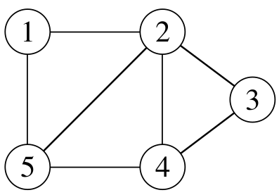
Graphs
- Two vertices are adjacent if they are joined by an edge.
- An edge connecting $u$ and $v$ is written $(u, v)$ and is said to be incident on vertices $u$ and $v$.
- A sequence $\langle v_1, v_2, \ldots, v_n \rangle$ forms a path of length $n - 1$ if there exist edges $(v_i, v_{i+1})$ for $1 \leq i < n$.
- The length of a path is the number of edges it contains.
There are two standard ways to represent a graph $G = (V, E)$:
- As adjacency lists: for each $u \in V$, adjacency list $Adj[u]$ contains vertices $\nu$ s.t. there is an edge $(u, \nu) \in E$.
- As adjacency matrix.
Graphs - Definitions
- In a directed graph, a path $ \langle v_0, v_1, \ldots, v_k \rangle$ forms a cycle if $v_0 = v_k$ and the path contains at least one edge.
- A cycle is simple if $ \langle v_1, v_2, \ldots, v_k \rangle$ are distinct.
- A self-loop is a cycle of length 1.
- An undirected graph is connected if every vertex is reachable from all other vertices.
- The connected components of a graph are the equivalence classes of vertices under the "is reachable from" relation.
- A directed graph is strongly connected if every two vertices are reachable from each other.
- The strongly connected components of a directed graph are the equivalence classes of vertices under the "are mutually reachable" relation.
- A directed graph is strongly connected if it has only one strongly connected component.
Graphs - Definitions
Two graphs $G=(V, E)$ and $G'=(V', E')$ are isomorphic if there exists a bijection $f: V \rightarrow V'$ such that $(u, v) \in E$ if and only if $(f(u), f(v)) \in E'$.
We say that a graph $G=(V, E)$ is a subgraph of
$G'=(V', E')$ if $V' \subseteq V$ and $E' \subseteq E$.
Given a set $V' \subseteq V$, the subgraph of $G$ induced
by $V'$ is the graph $G'=(V', E')$, where
$E'= \{(u,v) \in E : u,v \in V'\}$.
An undirected graph $G = (V, E)$
is bipartite if $V$ can be partitioned into
two sets $V_1$ and $V_2$ such that $(u, v) \in E$
implies either $u \in V_1$ and $v \in V_2$ or $u \in V_2$ and $v \in V_1$
Quiz (part 1)

5 minutes
Graphs (BFS)
Breadth-First Search explores in all possible directions:
- The visit starts from a source vertex $s$.
- Layer $L_1$ consists of all vertices that are neighbors of $s$.
- Layer $L_{j+1}$ consists of all vertices that do not belong to an earlier layer and have an edge to a vertex in $L_j$
For each $j \geq 1$, layer $L_j$ consists of all vertices at distance exactly $j$ from $s$. There is a path from $s$ to $t$ iff $t$ appears in some layer.
Breadth-First Search Algorithm
The algorithm can be written in pseudocode as: \begin{equation*} %\setlength\arraycolsep{1.5pt} \begin{array}{@{\quad}l} BFS(G, s) \\ \underline{In}: G=(V, E), s \in V \\ \underline{Out}: For ~ all ~ v \in V, return ~ distance~ v.d \\ s.d = 0 \quad // ~no~ driving~ to~ get~ here \\ for~all~u \in V \\ \quad u.d = \infty \quad //~ cannot~ get~ there \\ add(bag, s) \\ while~ bag~ not~ empty \\ \quad u=get(bag) \\ \quad for~all~(u,v) \in E \qquad \text{// visit neighbors next door }\\ \quad\quad if~v.d=\infty \\ \quad\quad\quad add(bag, v) \\ \quad\quad\quad v.d=u.d + 1 \end{array} \end{equation*}
Breadth-First Search Algorithm
The algorithm can be written in pseudocode as: \begin{equation*} %\setlength\arraycolsep{1.5pt} \begin{array}{@{\quad}l} BFS(G, s) \\ s.d = 0 \quad // ~no~ driving~ to~ get~ here \\ for~all~u \in V \\ \quad u.d = \infty; u.\pi = null \\ enqueue(queue, s) \\ while~queue~ not~ empty \\ \quad u=dequeue(queue) \\ \quad for~all~(u,v) \in E \qquad \text{// visit neighbors next door }\\ \quad\quad if~v.d=\infty \\ \quad\quad\quad enqueue(queue, v) \\ \quad\quad\quad v.d=u.d + 1; v.\pi = u \end{array} \end{equation*}
Quiz (part 2)

7 minutes
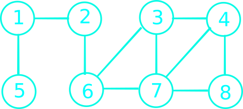
\begin{equation*} %\setlength\arraycolsep{1.5pt} \begin{array}{| c | c | c | c | c | c | c | c | } 1 & 2 & 3 & 4 & 5 & 6 & 7 & 8 \\\hline \quad & 0/null &\quad & \quad & \quad & \quad & \quad & \\ & & & & & & & \\ & & & & & & & \\ & & & & & & & \\ & & & & & & & \\ \end{array} \end{equation*}
Breadth-First Search Algorithm
The algorithm can be written in pseudocode as: \begin{equation*} %\setlength\arraycolsep{1.5pt} \begin{array}{@{\quad}l} BFS(G, s) \\ s.d = 0; s.color = pink; for~all~u \in V \\ \quad u.d = \infty; u.\pi = null \\ enqueue(queue, s) \\ while~queue~ not~ empty \\ \quad u=dequeue(queue) \\ \quad for~all~(u,v) \in E \qquad \text{// adjacent }\\ \quad\quad if~v.color=white \\ \quad\quad\quad v.color=pink \\ \quad\quad\quad enqueue(queue, v) \\ \quad\quad\quad v.d=u.d + 1; v.\pi = u \\ \quad u.color=red \\ \end{array} \end{equation*}

\begin{equation*} %\setlength\arraycolsep{1.5pt} \begin{array}{| l | c | c | c | c | c | c | c | c | } Q & 1 & 2 & 3 & 4 & 5 & 6 & 7 & 8 \\\hline 2 & \infty/n & 0/n & \infty/n & \infty/n & \infty/n & \infty/n & \infty/n & \infty/n \\ 1, 6 & 1/2 & 0/n & \infty/n & \infty/n & \infty/n & 1/2 & \infty/n & \infty/n \\ 6, 5 & 1/2 & 0/n & \infty/n & \infty/n & 2/1 & 1/2 & \infty/n & \infty/n \\ 5, 3, 7 & 1/2 & 0/n & 2/6 & \infty/n & 2/1 & 1/2 & 2/6 & \infty/n \\ 3, 7 & 1/2 & 0/n & 2/6 & \infty/n & 2/1 & 1/2 & 2/6 & \infty/n \\ 7, 4 & 1/2 & 0/n & 2/6 & 3/3 & 2/1 & 1/2 & 2/6 & \infty/n \\ 4, 8 & 1/2 & 0/n & 2/6 & 3/3 & 2/1 & 1/2 & 2/6 & 3/7 \\ 8 & 1/2 & 0/n & 2/6 & 3/3 & 2/1 & 1/2 & 2/6 & 3/7 \\ \emptyset & 1/2 & 0/n & 2/6 & 3/3 & 2/1 & 1/2 & 2/6 & 3/7 \\ \end{array} \end{equation*}
Welcome to CSC 282/482
Lecture 02.20

Correctness of BFS
Lemma 1
Let G=(V, E) be a directed or undirected graph, and let $s \in V$ be an arbitrary
vertex. Then, for any edge $(u, v) \in E$,
$\delta (s,v) \leq \delta(s,u) + 1$
Lemma 2
Let $G =(V, E)$ be a directed or undirected graph, and suppose that BFS is run
on $G$ from a given source vertex $s \in V$. Then upon termination,
for each vertex $\nu \in V$, the value $\nu.d$ computed by BFS satisfies $\nu.d \geq \delta(s,\nu)$
Lemma 3
Suppose that during the execution of BFS on a graph $G = (V, E)$, the queue $Q$
contains the vertices $\langle \nu_1, \nu_2, \ldots, \nu_r \rangle$, where $\nu_1$ is the head of $Q$
and $\nu_r$ is the tail.
Then, $\nu_r.d \leq \nu_1.d + 1$ and $\nu_i.d \leq \nu_{i+1}.d$ for $i = 1, 2, \ldots, r-1$.
Welcome to CSC 282/482
Lecture 02.22
Graphs (DFS)
Goal: Discover each reachable vertex in a graph.
Strategy: search "deeper" in the graph whenever possible.
- DFS explores edges out of the most recently discovered vertex $\nu$ that still has unexplored edges leaving it.
- when all of $\nu$'s edges have been explored, the search "backtracks" to explore edges leaving the vertex from which $\nu$ was discovered. process continues until we have discovered all the vertices that are reachable from the original source vertex.
- If any undiscovered vertices remain, then DFS selects one of them as a source, and it repeats the search from that source.
Graphs (DFS)
Goal: Discover each reachable vertex in a graph.
Strategy: search "deeper" in the graph whenever possible.

Graphs (DFS) - [CLRS]
The algorithm is given below:
Classification of edges
- Tree edges: are edges in the depth-first forest $G_\pi$.
- Back edges: are those edges connecting a vertex $u$ to an ancestor $v$ in a depth-first tree.
- Forward edges: are those nontree edges connecting a vertex $u$ to a descendant $v$ in a depth-first tree.
- Cross edges: are all other edges.
Shortest Path Problem

Shortest Path Problem
In a shortest-path problem we are given:
- A weighted, directed graph $G = (V, E)$.
- A weight function $w: E \rightarrow \mathbb{R}$
Definitions
- The weight of a path $p=\langle \nu_0,\nu_1, \ldots, \nu_k \rangle$ is: \begin{array}{c} w(p)=\sum_{i=1}^{k} w(\nu_{i-1}, \nu_i) \end{array}
- The shortest-path weight $\delta(u, \nu)$ from $u$ to $\nu$ \[ \delta(u, \nu) = \left\{ \begin{array}{ll} min\{ w(p): u \overset{p}{\rightsquigarrow} \nu \} & \mbox{if there is a path } u \mbox{ to } \nu \\ \infty & \mbox{otherwise.} \end{array} \right. \]
Dijkstra's Algorithm
The algorithm can be written in pseudocode as:
\begin{equation*} %\setlength\arraycolsep{1.5pt} \begin{array}{@{\quad}l} DIJKSTRA(G,w,s) \\ 1 \quad Initialize \\ 2 \quad Q=G.V\qquad // \text{ is this O(1)? } \\ 3 \quad while~ Q~ not~ empty \\ 4 \quad\quad u = extract\text{-}Min(Q) \\ 5 \quad\quad foreach ~ v \in G.Adj[u] \\ 6 \quad\quad\quad RELAX(u,v,w) \\ \end{array} \end{equation*}Dijkstra's Algorithm - Activity
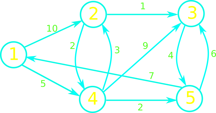
Thank you!
See you next time
Welcome to CSC 282/482
Lecture 02.27
Reminder: Homework posted.
Dijkstra's Algorithm - Activity
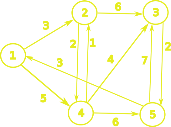
Bellman-Ford Algorithm (1955-1956)
The algorithm can be written in pseudocode as:
\begin{equation*} %\setlength\arraycolsep{1.5pt} \begin{array}{@{\quad}l} Bellman-Ford(G,w,s) \\ 1 \quad Initialize \\ 2 \quad for~i=1~to~|V| - 1 \quad\quad // \text{ why |V|-1? } \\ 3 \quad\quad foreach~(u,v) \in E \\ 4 \quad\quad \quad\quad relax(u, v, w) \\ 5 \quad foreach~(u,v) \in E \\ 6 \quad\quad if~v.d>u.d + w(u,v) \quad\quad // \text{ when does this occur? } \\ 7 \quad\quad\quad\quad return~false \\ 8 \quad return~true \end{array} \end{equation*}Bellman-Ford (Activity)
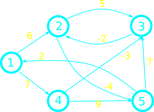
(1,2)(2,3)(3,2)(1,4)(4,3)(4,5)(2,5)(5,1)(5,3)
Thank you for the attention

Welcome to CSC 282/482
Lecture 02.29
Bellman-Ford (Activity)

(1,2)(2,3)(3,2)(1,4)(4,3)(4,5)(2,5)(5,1)(5,3)
Shortest Path Properties
Some important theorems follow:
- Triangle inequality: For any edge $(u, \nu) \in E$, $\delta(s, \nu) \leq \delta(s, u) + w(u, \nu)$
- Upper-bound: $\nu.d \geq \delta(s, \nu)$ for all $\nu \in V$ and once achieved it never changes.
- No-path: If no path from $s$ to $\nu$ , then $\nu.d = \delta(s, \nu) = \infty$
- Convergence: Suppose a sequence of relaxation steps including relax(u,v,w) is executed. If $s \cdots \rightarrow u \rightarrow \nu$ is a shortest path in G for some $(u, \nu) \in V$ and if $u.d = \delta(s,u)$ prior to relaxing edge $(u, \nu)$, then $\nu.d = \delta(s, \nu)$ at all times afterward.
- Path-relaxation: If $p = \langle \nu_0, \nu_1, \ldots, \nu_k \rangle$, is a shortest path with $s=\nu_0$, and we relax edges of $p$ in order, then $\nu_k.d = \delta(s, \nu_k)$.
Correctness of Bellman-Ford Algorithm
Lemma 2:
Let $G=(V, E)$ be a weighted, directed graph with source $s$.
Assume $G$ contains no negative-weight cycles that are
reachable from $s$.
After the $|V - 1|$ iterations of the for loop, we
have $\nu.d=\delta(s, \nu)$ for
all vertices $\nu$ that are reachable from $s$.
Theorem: Let $G=(V,E)$ be a directed weighted graph. Assume there are no negative-weight cycles.
Bellman-Ford will compute $v.d=\delta(s, v)$ for all $v \in V$.
Welcome to CSC 282/482
Lecture 03.05
Topological Ordering (Sorting)
Strongly-connected Components
Topological Ordering (Sorting)
- Task Scheduling: In project management, used to schedule tasks in a project where certain tasks depend on the completion of others.
- Dependency Resolution: In software development, used to resolve dependencies between modules, libraries, or packages.
- Instruction Scheduling: In compiler design, used for instruction scheduling in optimizing compilers. Instructions that are dependent on each other need to be scheduled in such a way that the dependencies are respected and execution efficiency is maximized.
- Data Dependency Analysis: In parallel computing and optimization, analyze data dependencies between different parts of a program or algorithm, to identify opportunities for parallelization and optimization.
- Network Routing: determine the order in which packets should be forwarded, to avoid loops, efficient delivery.
Topological Ordering
Many applications use directed acyclic graphs to indicate precedence among events.
A topological ordering of a dag $G = (V, E)$ is a linear ordering of all its vertices such that if $G$ contains an edge $(u,v)$, then $u$ appears before $v$ in the ordering.
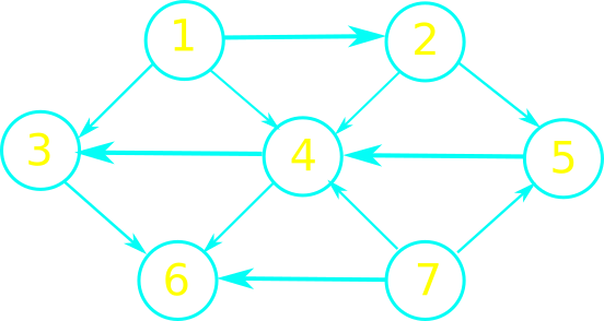 | 
|
Topological Ordering
A directed graph with no cycles is called directed acyclic graph, or a DAG for short.
A topological sort of a dag $G = (V, E)$ is a linear ordering of all its vertices such that if $G$ contains an edge $(u,v)$, then $u$ appears before $v$ in the ordering.
\begin{equation*} %\setlength\arraycolsep{1.5pt} \begin{array}{l} \text{TOPOLOGICAL-SORT(G)} \\ 1 \quad \text{call DFS(G) to compute finish times u.f} \\ 2 \quad \text{as each vertex is finished, insert it onto the front of a linked list} \\ 3 \quad \text{return the linked list of vertices} \\ \end{array} \end{equation*}
Topological Ordering - Toy Example

Strongly Connected Components
Very often graph algorithms start with a decomposition of a graph into its connected components.
For a directed graph $G=(V, E)$, a strongly connected component is a maximal set of vertices $C \in V$ such that for every pair of vertices $u$ and $v$ in $C$, vertices $u$ and $v$ are reachable from each other.
What are the strongly connected components of the following graph?
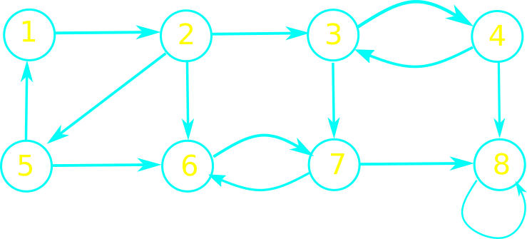
Strongly Connected Components - Algorithm
\begin{equation*} %\setlength\arraycolsep{1.5pt} \begin{array}{l} STRONGLY\text{-}CONNECTED\text{-}COMPONENTS(G) \\ 1 \quad call~ DFS(G)~ to~ compute~ finishing~ times~ u.f \\ 2 \quad compute~ G^T \\ 3 \quad call~ DFS(G^T),~ but~ in~ the ~main~ loop~ of~ DFS,~ consider~ the~ vertices~ in~ order~ of~ decreasing~ u.f \\ 4 \quad output~ vertices~ of~ DFS~ trees~ in~ line~ 3~ as~ a~ separate~ s.c.c \\ \end{array} \end{equation*}
SCC - Toy Example
Find the strongly connected components of the following graph:
 | \begin{equation*} %\setlength\arraycolsep{1.5pt} \begin{array}{l} \text{STRONGLY-CONNECTED-COMPONENTS(G)} \\ 1 \quad \text{call DFS(G) to compute finish times u.f} \\ 2 \quad \text{compute}~G^T \\ 3 \quad \text{call}~DFS(G^T)\text{, but consider the vertices in order of decreasing u.f} \\ 4 \quad \text{output vertices of DFS trees in line 3 as a separate s.c.c} \\ \end{array} \end{equation*} |
SCC - Toy Example
Find the strongly connected components of the following graph:
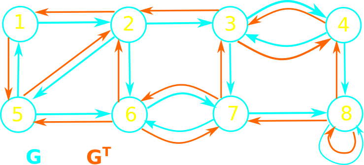
Quiz Break

Thank you!
See you next time
Welcome to CSC 282/482 (04.02.2024)
Introduction to Linear Programming
- Reminder: Last HW posted
- Notation
- Geometric Representation*
- Standard Form
* Ἀγεωμέτρητος μηδεὶς εἰσίτω (Plato)
Linear Programming Problems
Problems that model situations involving resources and activities.
Resources
- Money
- Equipment
- Personnel
Activities
- Investing in projects
- Shipping of goods
- Advertising in media
Goal: Allocate resources to activities to achieve the best possible value of performance.
Linear Programming Problems (Toy 1)
Kantina Dukat produces high-quality wine and raki*.
\begin{equation*} %\setlength\arraycolsep{1.5pt} \begin{array}{c@{\quad}| c c c} Operation & Vlosh & Moskat & Production Time \\\hline Harvest & 1 & 0 & 4 \\ Fermentation & 0 & 2 & 12 \\ Distillation & 3 & 2 & 18 \\ Profit ~(lekë) & 3000 & 5000 & \\ \end{array} \end{equation*}
The management wishes to determine the quantities for the two drinks in order to maximize their total profit, subject to the restrictions imposed by the capacities above.
* Drink made out of grapes or other fruits.
Linear Programming Problems (Toy 2)
Assume the following models a problem with two decision variables: \begin{equation*} %\setlength\arraycolsep{1.5pt} \begin{array}{l@{\quad} r c r c r} \max & x_1 & + & x_2 & & \\ \mathrm{s.t.} & 4x_1 & - & x_2 & \leq & 8 \\ & 2x_1 & + & x_2 & \leq & 10 \\ & 5x_1 & - & 2x_2 & \geq & -2 \\ & & & x_1,x_2 & \geq & 0 \end{array} \end{equation*}
Any assignment of the $x_1$ and $x_2$ that satisfies all the constraints is a feasible solution to the linear program.
Standard form
The standard form of a linear program is given by:
- $n$ real numbers $c_1,c_2, \ldots, c_n$
- $m$ real numbers $b_1,b_2, \ldots, b_m$
- $mn$ real numbers $a_{ij}$ for i = $1, 2,\ldots, m$ and j = $1, 2,\ldots, n$.
We wish to find $n$ real numbers $x_1,x_2, \ldots, x_n$ that \begin{equation*} %\setlength\arraycolsep{1.5pt} \begin{array}{l@{\quad} l c r c r} maximize & Z=\sum_{j=1}^{n} c_j x_j & \\ subject~to & \sum_{j=1}^{n} a_{ij} x_j \leq b_i & for~i=1,2,\ldots,m \\ & x_j \geq 0 & for~j=1,2,\ldots,n \\ \end{array} \end{equation*}
Converting into standard form
It is always possible to convert a linear program into standard form.
- The objective function might be a minimization rather than a maximization.
- There might be variables without nonnegativity constraints.
- There might be equality constraints, which have an equal sign rather than a less-than-or-equal-to sign.
- There might be inequality constraints, but instead of having a less-than-or- equal-to sign, they have a greater-than-or-equal-to sign.
Thank you for the attention
References:
- [CLRS] Introduction to Algorithms (29.1)
- Kantorovich, L.V. (1939). "Mathematical Methods of Organizing and Planning Production". Management Science. 6 (4): 366–422.
- Dantzig, George, Linear programming and extensions. Princeton University Press and the RAND Corporation, 1963.
Welcome to CSC 282/482 (04.04)
Slack Form for Linear Programs
Simplex Method
Converting into slack form
For certain purposes we prefer the slack form in which some of the constraints are equality constraints.
Let \begin{equation*} %\setlength\arraycolsep{1.5pt} \begin{array}{l@{\quad} r } \sum_{j=1}^{n} a_{ij} x_j \leq b_i \end{array} \end{equation*} be some inequality constraints. We introduce a new variable $s$ and rewrite the former as \begin{equation*} %\setlength\arraycolsep{1.5pt} \begin{array}{l@{\quad} r } s = b_i - \sum_{j=1}^{n} a_{ij} x_j \\ s \geq 0 \end{array} \end{equation*}
We call $s$ a slack variable as it measures the difference between the left-hand and right-hand sides in the former equation.
From standard form to slack form
[CLRS] notation: When converting from standard to slack form, it uses $x_{n+i}$ (instead of $s$) to denote the slack variable associated with the $i$th inequality. \begin{equation*} %\setlength\arraycolsep{1.5pt} \begin{array}{l@{\quad} r } x_{n+i} = b_i - \sum_{j=1}^{n} a_{ij} x_j \\ x_{n+i} \geq 0 \end{array} \end{equation*}
Slack Form (Toy 1)
A given linear program in standard form can be converted into slack form.
Maximize $Z = 2x_1 - 3x_2 + 3x_3$
| \begin{equation*} %\setlength\arraycolsep{1.5pt} \begin{array}{l@{\quad} r c r c r c r} % \max & x_1 & + & x_2 & & \\ \mathrm{s.t.} & x_1 & + & x_2 & - & x_3 & \leq & 7 \\ & -x_1 & - & x_2 & + & x_3 & \leq & -7 \\ & x_1 & - & 2x_2 & + & 2x_3 & \leq & 4 \\ & & & x_1,x_2, x_3 & \geq & 0 & & \end{array} \end{equation*} |
Quiz Break

Simplex Method (Dantzig 1947)
Notation: We'll use $\sum_{j=1}^{n} a_{ij} x_j + s_i = b_i$ and the simplex tableau, consisting of the augmented matrix corresponding to the constraint equations together with the coefficients of the objective function in the form:
Maximize $Z = 4x_1 + 6x_2$
| \begin{equation*} %\setlength\arraycolsep{1.5pt} \begin{array}{r c r c r } -x_1 & + & x_2 & \leq & 11 \\ x_1 & + & x_2 & \leq & 27 \\ 2x_1 & + & 5x_2 & \leq & 90 \\ x_1, & x_2 & \geq & 0 & \end{array} \end{equation*} | \begin{array}{c@{\quad} c@{\quad} c@{\quad} c@{\quad} c@{\quad} c@{\quad}c} x_1 & x_2 & s_1 & s_2 & s_3 & b \\\hline -1 & 1 & 1 & 0 & 0 & 11 \\ 1 & 1 & 0 & 1 & 0 & 27 \\ 2 & 5 & 0 & 0 & 1 & 90 \\\hline -4 & -6 & 0 & 0 & 0 & 0 \end{array} |
Simplex Method (Dantzig 1947)
To solve a linear programm problem in standard form, follow:
- Convert to slack form.
- Fill in the initial simplex tableau.
- Locate the most negative entry in the bottom row. That column is called entering column.
- Take ratios of entries in the “b-column” with their corresponding positive entries in the entering column. The leaving row is the smallest non- negative ratio $b_i / a_{ij}$. The entry in the leaving row and the entering column is called the pivot.
- Use row operations so that the pivot is 1, and all other entries in the entering column are 0.
- If all entries in the bottom row are zero or positive, this is the final tableau. If not, go back to Step 3.
- If you obtain a final tableau, then the linear programming problem has a maximum solution, which is given by the entry in the lower-right corner of the tableau.
Thank you for the attention
References:
- [CLRS] Introduction to Algorithms (29.3)
- Kantorovich, L.V. (1939). "Mathematical Methods of Organizing and Planning Production". Management Science. 6 (4): 366–422.
- Dantzig, George, Linear programming and extensions. Princeton University Press and the RAND Corporation, 1963.
Thank you for the attention

😎
Thank you!
Welcome to CSC 282/482 (04.09.2024)
More Simplex Examples
Artificial Variables
Applications
Applications
Simplex with Three Variables (Toy 1)
Find the maximum value of $z=2x_1 - x_2 + 2x_3$.
| Subject to \begin{array}{c@{\quad} c@{\quad} c@{\quad} c@{\quad} c@{\quad} c@{\quad}c} 2x_1 & + & x_2 & & & \leq & 10 \\ x_1 & + & 2x_2 & - & 2x_3 & \leq & 20 \\ & & x_2 & + & 2x_3 & \leq & 5 \\ & & x_1, & x_2, & x_3, & \geq & 0 \\ \end{array} |
\begin{array}{c@{\quad} c@{\quad} c@{\quad} c@{\quad} c@{\quad} c@{\quad} c@{\quad}|c} x_1 & x_2 & x_3 & s_1 & s_2 & s_3 & b & Base \\\hline & & & & & & & s_1\\ & & & & & & & s_2 \\ & & & & & & & s_3 \\\hline \end{array} |
Simplex with Artificial Variable (Toy 2)
Find the maximum value of $z=3x_1 + 2x_2 + x_3$.
| Subject to \begin{array}{c@{\quad} c@{\quad} c@{\quad} c@{\quad} c@{\quad} c@{\quad}c} 4x_1 & + & x_2 & + & x_3 & = & 30 \\ 2x_1 & + & 3x_2 & + & x_3 & \leq & 60 \\ x_1 & + & 2x_2 & + & 3x_3 & \leq & 40 \\ & & x_1, & x_2, & x_3, & \geq & 0 \\ \end{array} |
\begin{array}{c@{\quad} c@{\quad} c@{\quad} c@{\quad} c@{\quad} c@{\quad} c@{\quad}|c} x_1 & x_2 & x_3 & s_1 & s_2 & s_3 & b & Base \\\hline & & & & & & & s_1\\ & & & & & & & s_2 \\ & & & & & & & s_3 \\\hline \end{array} |
Aluminium Windows and Doors (1)
URDoor produces aluminium windows and doors.
\begin{equation*} %\setlength\arraycolsep{1.5pt} \begin{array}{|l| c c c c | } \hline Process & Window & Door & Accessories & Time Available \\\hline Molding & 1 & 2 & 3/2 & 12000 \\ Trimming & 2/3 & 2/3 & 1 & 4600 \\ Packaging & 1/2 & 1/3 & 1/2 & 2400 \\ Profit & 11 & 16 & 15 & - \\\hline \end{array} \end{equation*}
Profit is $Z=11x_1 + 16x_2 + 15x_3$Aluminium Windows and Doors (2)
|
\begin{array}{c@{\quad} c@{\quad} c@{\quad} c@{\quad} c@{\quad} c@{\quad}c} x_1 & + & 2x_2 & + & \frac{3}{2}x_3 & \leq & 12000 \\ \frac{2}{3}x_1 & + & \frac{2}{3}x_2 & + & x_3 & \leq & 4600 \\ \frac{1}{2}x_1 & + & \frac{1}{3}x_2 & + & \frac{1}{2}x_3 & \leq & 2400 \\ \end{array} |
\begin{array}{c@{\quad}| c@{\quad}| c@{\quad}| c@{\quad}| c@{\quad}| c@{\quad}| c@{\quad}|c}
x_1 & x_2 & x_3 & s_1 & s_2 & s_3 & \quad b \quad & Base \\\hline
& & & & & & & s_1\\
& & & & & & & s_2 \\
& & & & & & & s_3 \\\hline
\end{array}
\begin{array}{c@{\quad} c@{\quad} c@{\quad} c@{\quad} c@{\quad} c@{\quad} c@{\quad}|c} x_1 & x_2 & x_3 & s_1 & s_2 & s_3 & b & Base \\\hline 1 & 2 & \frac{3}{2} & 1 & 0 & 0 & 12000 & s_1\\ \frac{2}{3} & \frac{2}{3} & 1 & 0 & 1 & 0 & 4600 & s_2 \\ \frac{1}{2} & \frac{1}{3} & \frac{1}{2} & 0 & 0 & 1& 2400 & s_3 \\\hline -11 & -16 & -15 & 0 & 0 & 0 & 0 & \\ \end{array} |
Thank you for the attention

Welcome to CSC 282/482 (04.11.2024)
Gauss and Gauss-Jordan Elimination Method
Duality
Systems of Linear Equations
Assume you are given the following linear equations to solve:
\begin{array}{r@{\quad} c@{\quad} r@{\quad} c@{\quad} c@{\quad} r@{\quad}r c | c r@{\quad} c@{\quad} r@{\quad} c@{\quad} r@{\quad} c@{\quad}r} x & - & 2y & + & 3z & = & 9 & & & x & - & 2y & + & 3z & = & 9\\ -x & + & 3y & & & = & -4 & & & & & y & + & 3z & = & 5 \\ 2x & - & 5y & + & 5z & = & 17 & & & & & & & z & = & 2 \\ \end{array}
Which one is easier to solve?
Systems of Linear Equations
Which one is easier to solve?
\begin{array}{r@{\quad} c@{\quad} r@{\quad} c@{\quad} c@{\quad} r@{\quad}r c | c r@{\quad} c@{\quad} r@{\quad} c@{\quad} r@{\quad} c@{\quad}r} x & - & 2y & + & 3z & = & 9 & & & x & - & 2y & + & 3z & = & 9\\ -x & + & 3y & & & = & -4 & & & & & y & + & 3z & = & 5 \\ 2x & - & 5y & + & 5z & = & 17 & & & & & & & z & = & 2 \\ \end{array}
We can transform a system of linear equations into an equivalent one using row-operations:
1. Interchange two equations.
2. Multiply an equation by a nonzero constant.
3. Add a multiple of an equation to another equation.
Row-Echelon Form
A matrix in row-echelon form has the following properties:
1. All rows consisting entirely of zeros occur at the bottom of the matrix.
2. For each row that does not consist entirely of zeros, the first nonzero entry is 1.
3. For two successive (nonzero) rows, the leading 1 in the
higher row is farther to the left than the leading 1 in the lower row.
A matrix in row-echelon form is in reduced row-echelon form
if every column that has a leading 1 has zeros in every position above and below its leading 1.
Gaussian Elimination
1. Write the augmented matrix of the system of linear equations.
2. Use elementary row operations to rewrite the augmented matrix in row-echelon form.
3. Write the system of linear equations corresponding to the matrix in row-echelon form,
and use back-substitution to find the solution.
Solve the system \begin{array}{c@{\quad} c@{\quad} c@{\quad} c@{\quad} c@{\quad} c@{\quad} c@{\quad} c@{\quad} c@{\quad}} & & x_2 & + & x_3 & - & 2x_4 & = & -3 \\ x_1 & + & 2x_2 & - & x_3 & & & = & 2 \\ 2x_1 & + & 4x_2 & + & x_3 & - & 3x_4 & = & -2 \\ x_1 & - & 4x_2 & - & 7x_3 & - & x_4 & = & -19 \\ \end{array}
Quiz Break

Duality
Given a linear program with an objective function to maximize, we can transform it into a minimization problem with the same optimal solution.
Minimize $z=0.12x_1 + 0.15x_2$. Subject to \begin{array}{c@{\quad} c@{\quad} c@{\quad} c@{\quad} c@{\quad} c@{\quad}c} 60x_1 & + & 60x_2 & \geq & 300 \\ 12x_1 & + & 6x_2 & \geq & 36 \\ 10x_1 & + & 30x_2 & \geq & 90 \\ \end{array}
\begin{equation} \left[ \begin{array}{c@{\quad} c@{\quad}: c@{\quad}} 60 & 60 & 300 \\ 12& 6 & 36 \\ 10 & 30 & 90 \\\hdashline 0.12 & 0.15 & 0 \\ \end{array} \right] \end{equation}
From Primal to Dual
Minimize $z=0.12x_1 + 0.15x_2$. Subject to \begin{array}{c@{\quad} c@{\quad} c@{\quad} c@{\quad} c@{\quad} c@{\quad}c} 60x_1 & + & 60x_2 & \geq & 300 \\ 12x_1 & + & 6x_2 & \geq & 36 \\ 10x_1 & + & 30x_2 & \geq & 90 \\ \end{array}
\begin{equation} \left[ \begin{array}{c@{\quad} c@{\quad}: c@{\quad}} 60 & 60 & 300 \\ 12& 6 & 36 \\ 10 & 30 & 90 \\\hdashline 0.12 & 0.15 & 0 \\ \end{array} \right] \end{equation}
Maximize $z=\quad y_1 + \quad y_2 + \quad y_3$, subject to \begin{array}{c@{\quad} c@{\quad} c@{\quad} c@{\quad} c@{\quad} c@{\quad}c} \quad y_1 & + & \quad y_2 & + & \quad y_3 & \quad & \quad \\ \quad y_1 & + & \quad y_2 & + & \quad y_3 & \quad & \quad \\ \end{array}
\begin{equation} \left[ \begin{array}{c@{\quad} c@{\quad} c@{\quad}: c@{\quad}} \quad & \quad & \quad & \quad \\ \quad & \quad & \quad & \quad \\\hdashline \quad & \quad & \quad & \quad \\ \end{array} \right] \end{equation}
Thank you for the attention
 (thetartan.org)
References:
- [CLRS] Introduction to Algorithms (29.4)
- Gauss-Jordan Resources
Welcome to CSC 282/482 (04.16.2024)
Divide and Conquer Algorithms
Counting Inversions
Closest Pair of Points
Divide and Conquer (memento)
The divide and conquer algorithmic technique has three steps:
- Divide the initial problem in smaller parts (subproblems)
- Solve (conquer) each subproblem recursively
- Combine solutions to subproblems to get the solution of the original problem
Typical examples include: mergesort, quicksort, binary search, tree operations, Hanoi Towers solutions, etc.
How (dis)similar?
Application: Collaborative filtering
- Matches preference of users (books, music, movies, restaurants) with that of others
- Finds people with similar tastes
- Recommends new things to users based on purchases of these people
Goal: compare the similarity of two rankings.
Consider the following scenario:
- Alice is asked to give a list of her favorite movies in order of preference.
- Bob is asked to give a list of his favorite movies in order of preference.
How "similar" are their tastes?
Counting Inversions - The Problem
Input: A sequence of $n$ numbers $a_1, \ldots , a_n$.
- We want to define a measure that tells us how far this list is from being in ascending order.
- Should be $0$ if $a_1 < a_2 < \ldots < a_n$, and should increase as the numbers become more scrambled.
- A natural way to quantify this notion is by counting the number of inversions.
- We say that two indices $i < j$ form an inversion if $a_i > a_j$.
Goal: Determine the number of inversions in the sequence $a_1, \ldots , a_n$.
\begin{equation}
\begin{array}{| c@{\quad} | c@{\quad} | c@{\quad} | c@{\quad} | c@{\quad} | c@{\quad} |}
\hline
1 & 3 & 5 & 2 & 4 & 6 \\\hline
\end{array}
\end{equation}
\begin{equation}
\begin{array}{| c@{\quad} | c@{\quad} | c@{\quad} | c@{\quad} | c@{\quad} | c@{\quad} |}
\hline
1 & 2 & 3 & 4 & 5 & 6 \\\hline
\end{array}
\end{equation}
Counting Inversions - Solution
We can try to apply the divide and conquer approach:
- Divide the sequence in two parts.
- What next? ...
Counting Inversions - Solution
We can try to apply the divide and conquer approach:
- Divide the sequence in two parts.
- Count the number of inversions in each of the parts.
- Count inversions $(a_i , a _j)$, where $a_i$ and $a_j$ in different parts.
- Combine results from subproblems (sum of 2 and 3)
Closest Pair of Points (Notation)
Input: $n \geq 2$ points (plane) from a set of points $P$
Output: Pair of points with the smallest Euclidean distance.
Definitions:
- The Euclidean distance is defined as $d(p_1, p_2) = \sqrt{(x_1 - x_2)^2 + (y_1 - y_2)^2}$
- Two points $p_1$, $p_2$ are coincident if $d(p_1, p_2) = 0$
Typical applications include: traffic-control systems, robotics, computer vision, etc.
Closest Pair of Points (Algorithm)
Each recursive step takes as input
- a subset $P \subseteq Q$
- arrays $X$ and $Y$, each of which contains all the points of $P$.
- points in $X$ are sorted by monotonically increasing $x$-coordinates.
- array $Y$ is sorted by monotonically increasing $y$-coordinate.
Closest Pair of Points (Divide)
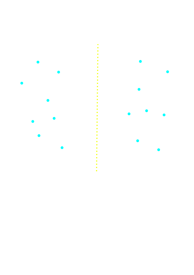
-
Find a vertical line $l$ that bisects the point set $P$ into two sets $P_L$ and $P_R$,
with $|P_L| = \lceil |P|/2 \rceil$ and $|P_R| = \lfloor |P|/2 \rfloor$
- all points in $P_L$ are on or to the left of line $l$, and all points in $P_R$ are on or to the right of $l$.
- divide the array $X$ into arrays $X_L$ and $X_R$, which contain the points of $P_L$ and $P_R$ respectively, sorted by monotonically increasing x-coordinate.
- divide the array $Y$ into arrays $Y_L$ and $Y_R$, which contain the points of $P_L$ and $P_R$ respectively, sorted by monotonically increasing y-coordinate.
Closest Pair of Points (divide)
Closest Pair of Points (Conquer)
- Recursively find the closest pair of points in $P_L$, return $\delta_L$.
- Recursively find the closest pair of points in $P_R$, return $\delta_R$.
- $\delta = min(\delta_L, \delta_R)$
Combine
- The closest pair is the pair with distance $\delta$ found by one of the recursive calls. Right?
Closest Pair of Points (Conquer)
- Recursively find the closest pair of points in $P_L$, return $\delta_L$.
- Recursively find the closest pair of points in $P_R$, return $\delta_R$.
- $\delta = min(\delta_L, \delta_R)$
Combine
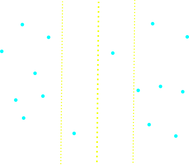
- The closest pair is the pair with distance $\delta$ found by one of the recursive calls OR
- It is a pair of points with one point in $P_L$ and the other in $P_R$. The algorithm determines whether there is a pair with one point in $P_L$ and the other point in $P_R$ and whose distance is less than $\delta$.
Closest Pair of Points (Splits)
Closest Pair of Points (Combine)
- Create an array $Y'$, as the array Y with only points in the $2\delta$-wide vertical strip. The array $Y'$ is sorted by y-coordinate.
- For each point $p$ in the array $Y'$, find points in $Y'$ that are within $\delta$ units of $p$. Keep track of the closest-pair distance $\delta'$ found over all pairs of points in $Y'$. If $\delta' < \delta$, then return the respective pair and its distance $\delta'$. Otherwise, return the closest pair and its distance $\delta$ found by the recursive calls.
Thank you for the attention

References:
- [CLRS] Introduction to Algorithms (33.4)
- [KT] Algorithm Design 5.3, 5.4
Welcome to 282 (04.18)
Computational Geometry Problems
Convex Hull
Robot Motion
Find the shortest path from $s$ to $t$ that avoids the obstacle.

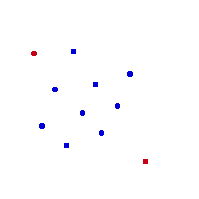
Farthest Pair
Given a set of points in the plane, find the farthest pair of points.
Convex Hull (Definition)
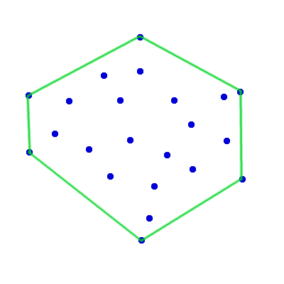
The convex hull of a set of points $Q$, denoted with $CH(Q)$ is the smallest convex polygon $P$ for
which each point in $Q$ is either on the boundary of $P$ or in its interior.
Graham's Scan (Idea - Ronald Graham '72)
Solves the problem by maintaining a stack:
- each point is pushed onto the stack once
- pop from the stack point that is not a vertex of CH(Q)
- upon termination the stack contains all vertices of CH(Q).
Graham's Scan
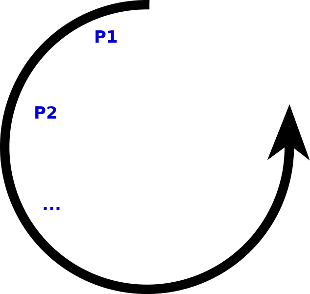
Points are traversed in order of increasing polar angle with respect to the starting point $p_0$
define polar angle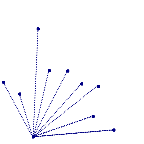
Graham's Scan
\begin{equation*} %\setlength\arraycolsep{1.5pt} \begin{array}{rl} GS(Q) \\ 1&Init~ p_0 \\ 2&Sort~points~by~polar~angle \\ 3&Init~stack~ S \\ 4&push(S, p_0) \\ 5&push(S, p_1) \\ 6&push(S, p_2) \\ 7&for~ i=3~ to~ m \\ 8&\quad while~ angle~ formed~ by ~next(S), top(S), p_i~nonleft~turn \\ 9&\quad\quad \quad pop(S) \\ 10&\quad push(S,p_i) \\ 11&return~S \end{array} \end{equation*}
Voronoi Diagram
Given a finite set of points $\{p_1,\ldots, p_n\}$ in the Euclidean plane. The cell $R_k$ for the point $p_k$ consists of every point in the Euclidean plane whose distance to $p_k$ is less than or equal to its distance to any other $p_k$.
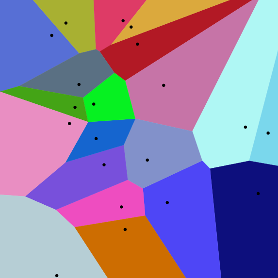
Used in biology, ecology, computational chemistry, medical diagnosis, epidemiology, materials science, urban planning, networking, computer graphics, machine learning, etc.
Delaunay Triangulation
Given a set of points in a plane is find a triangulation such that no point is inside the circumcircle of any triangle.
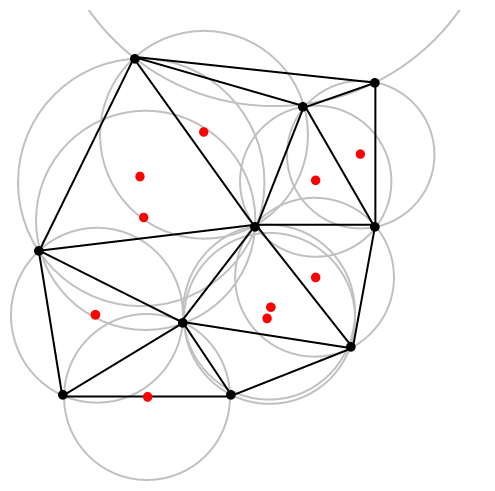
Used in path planning, terrain modelling, automated driving, simulations, etc.
Polar Angle Definitions ("stolen" from Wolfram)
In the plane, the polar angle $\theta$ is the counterclockwise angle from the $x$-axis at which a point in the $xy$-plane lies.
Such angle $\theta$ is usually measured in radians. The radian is a unit of angular measure defined such that an angle of one radian subtended from the center of a unit circle produces an arc with arc length $1$.
A full angle is therefore $2\pi$ radians, so there are 360 degrees per $2\pi$ radians, equal to 180 degrees/$\pi$ or 57.29577951 degrees/radian.
https://mathworld.wolfram.com/Angle.htmlConvex Polygon ("stolen" from Wolfram)
A planar polygon is convex if it contains all the line segments connecting any pair of its points. Thus, for example, a regular pentagon is convex (left figure), while an indented pentagon is not (right figure).
A planar polygon that is not convex is said to be a concave polygon.
Check left-turn, right-turn
Consider three points: $P_1$, $P_2$ and $P_3$. We have to decide whether $P_1P_2P_3$ represents a "right turn" (i.e. a turn in clockwise order) or a "left turn" (i.e. a turn in counter-clockwise order).
Given $P_1=(x_1,y_1)$, $P_2=(x_2,y_2)$ and $P_3=(x_3,y_3)$, we compute $(x_2−x_1)(y_3−y_1)−(y_2−y_1)(x_3−x_1)$:
- If the result is $0$, the points $P_1$, $P_2$ and $P_3$ are collinear.
- If the result is positive, the three points constitute a "left turn" (or a counter-clockwise orientation),
- otherwise the points represent a "right turn" (or a clockwise orientation). This reasoning assumes counter-clockwise numbered points.
Thank you for the attention

References:
- [CLRS] Introduction to Algorithms (33.3)
- Graham, R.L. (1972). "An Efficient Algorithm for Determining the Convex Hull of a Finite Planar Set"
- Visualizing the Connection Among Convex Hull,Voronoi Diagram and Delaunay Triangulation
Welcome to CSC 282/482 (04.23.2024)
Multiplication of Numbers
Multiplication of Matrices
Multiplication in Subquadratic Time
Multiplication of Numbers: Back to Grade School
Input: Two $n$-digit nonnegative integers, $x$ and $y$.
Output: The product $x \cdot y$
How many primitive operations? (Asymptotic Notation is fine) add quiz
Multiplication of Numbers: Can we do better?

Multiplication of Numbers - Let's break it down
Idea: Let's "cut" our numbers into parts.
Suppose $x$ and $y$ are $n$-bit integers. We need to compute the product $x \cdot y$.
- Split each of them into left and right parts: $x_L$, $x_R$, $y_L$, $y_R$
- $x=2^{n/2}x_L + x_R$
- $y=2^{n/2}y_L + y_R$
Multiplication of Numbers - The history (1)
Andrei Kolmogorov, one of the giants of $20$th century mathematics, conjectured that "there is no algorithm to multiply two $n$-digit numbers in subquadratic time". In 1960 (Moscow University) he restates his “$n^2$ conjecture” and posed several related problems.

Multiplication of Numbers - The history (2)
About a week later, a 23-year-old student named Anatolii Karatsuba presented Kolmogorov with a remarkable counterexample: multiplication in $O(n^{log_2 3})$ time.

Matrix Multiplication (1)
Suppose $X$ and $Y$ are $n \times n$ matrices of integers. In the product $Z=X \cdot Y$, entry $z_{ij}$ is the (dot) product of $i$th row of $X$ and $j$th column of $Y$: \begin{equation} z_{ij} = \sum_{k=1}^n x_{ik} y_{kj} \end{equation}
What would be the running time of a *naive* algorithm for computing the product?

Matrix Multiplication: Naive Algorithm
Suppose $X$ and $Y$ are $n \times n$ matrices of integers. In the product $Z=X \cdot Y$, entry $z_{ij}$ is the (dot) product of $i$th row of $X$ and $j$th column of $Y$:
\begin{equation} \begin{array}{l} \hline \text{Input: Two matrices $X$ and $Y$} \\ \text{Output: The matrix product $X \cdot Y$} \\ \hline \text{for $i=1$ to $n$ do} \\ \quad \text{for $j=1$ to $n$ do} \\ \quad \quad Z[i][j]=0 \\ \quad \quad \text{for $k=1$ to $n$ do} \\ \quad \quad \quad Z[i][j] = Z[i][j] + X[i][k] * Y[k][j] \\ \text{return $Z$} \end{array} \end{equation}
Divide and Conquer?
Idea: Divide a square matrix to smaller square submatrices.
| \begin{equation} X = \begin{pmatrix} A & B \\ C & D \end{pmatrix} \end{equation} | \begin{equation} Y = \begin{pmatrix} E & F \\ G & H \end{pmatrix} \end{equation} | \begin{equation} Z= X \cdot Y = \begin{pmatrix} A \cdot E + B \cdot G & A \cdot F + B \cdot H \\ C \cdot E + D \cdot G & C \cdot F + D \cdot H \end{pmatrix} \end{equation} |
with $A, B, \ldots, H$ all $\frac{n}{2} \times \frac{n}{2}$ matrices.
Divide and Conquer: First Algorithm
Idea: Divide a square matrix to smaller square submatrices
\begin{equation} \begin{array}{l} \hline \text{Input: Two matrices $X$ and $Y$} \\ \text{Output: The matrix product $Z=X \cdot Y$} \\ \hline \text{if $n=1$ then} \\ \quad \text{return $1 \times 1$ matrix with $X[1][1] * Y[1][1]$} \\ \text{else} \\ \quad \text{Set $A, B, C, D$ as submatrices of X} \\ \quad \text{Set $E, F, G, H$ as submatrices of Y} \\ \quad \text{recursively compute the $8$ matrix products} \\ \quad \text{return result of the computation} \end{array} \end{equation}
Strassen's Algorithm
Idea: Save one recursive call in exchange for additional matrix additions/subtractions.
Strassen's Algorithm (1969)
Idea: Save one recursive call in exchange for additional matrix additions/subtractions.
\begin{equation} \begin{array}{l} \hline \text{Input: Two matrices $X$ and $Y$} \\ \text{Output: The matrix product $Z=X \cdot Y$} \\ \hline \text{if $n=1$ then} \\ \quad \text{return $1 \times 1$ matrix with $X[1][1] * Y[1][1]$} \\ \text{else} \\ \quad \text{Set $A, B, C, D$ as submatrices of X} \\ \quad \text{Set $E, F, G, H$ as submatrices of Y} \\ \quad \text{recursively compute the $7$ products $P_i$} \\ \quad \text{return result of the additions/subtractions involving $P_i$(s)} \end{array} \end{equation}
Thank you for the attention

- Knuth, Donald E. (1988), The Art of Computer Programming volume 2: Seminumerical algorithms, Addison-Wesley, pp. 519, 706
- A. Karatsuba and Yu. Ofman (1962). "Multiplication of Many-Digital Numbers by Automatic Computers". Proceedings of the USSR Academy of Sciences. 145: 293–294
- A. A. Karatsuba (1995). "The Complexity of Computations" (PDF). Proceedings of the Steklov Institute of Mathematics. 211: 169–183. Translation from Trudy Mat. Inst. Steklova, 211, 186–202 (1995)
- Algorithms Illuminated - Tim Roughgarden
- [CLRS] - 4.2
- [DPV] - 2.1
- [Erickson] - Chapter 1