Sorting

Weiss Ch. 7

Important application, much analyzed, many algorithms. Arguably "simplest" for those who haven't bought into recursion are the O(N²) sorts, but quicksort is also very natural and illustrates divide and conquer with O(NlogN) time, which we can prove is the fastest we can do general sorting (based on elementwise comparisons).

Weiss uses java Comparators to decide the sorted order of two elements.

Bubble Sort

"My first sort", not in Weiss, sort of is in our

Sorting PPT.

I like:
Wikipedia.

O(N²): very similar to insertion sort.

Insertion Sort

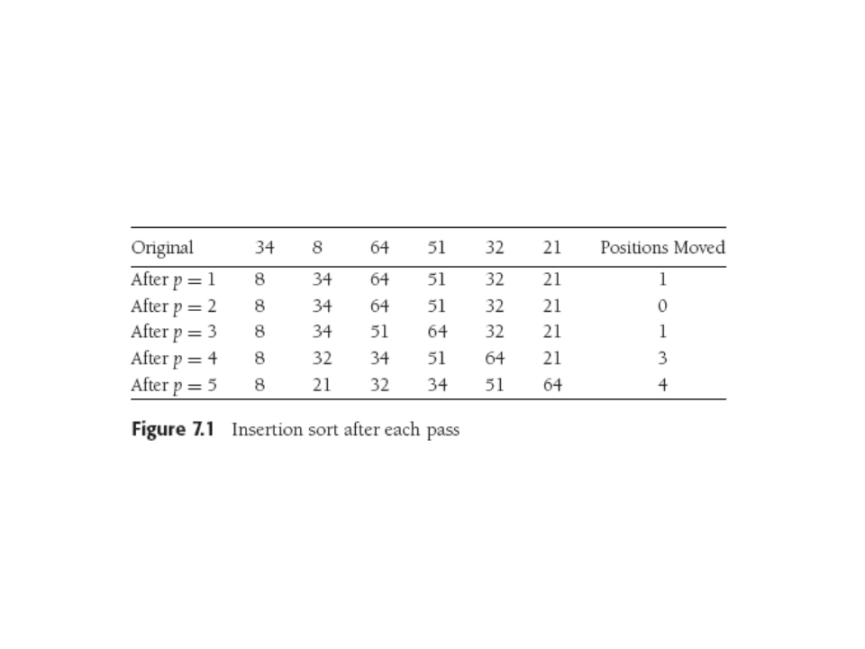
N-1 passes thru array, pass p = 1 thru N-1. After the pth pass, items 0-p are in sorted order. Move element in position p left until in right spot, REMEMBERING that everything to the left is already sorted (so can quit early).

Wikipedia.

Worst-case and expected time O(N²) by nested N-long for loops, but more exactly get N(N-1)/2, or sum of 1 to N. Best case is pre-sorted input (not true for all sorts!): the sort just checks the order and never does any swapping, so O(N).

Lower bound for simple sorting

Inversion: an out-of-order ordered pair of numbers in an array, as
1 2 4 3 (one inversion) 4 1 2 3 (three inversions). Swapping two out-of-order, adjacent elements removes exactly one inversion.

In insertion sort, O(N) other work plus O(I) swaps with I inversions, so O(N+I), or O(N) if there are O(N) inversions.

Could get average running time by computing average number of inversions in a permutation (of first N ints, no duplicates).

Theorem 7.1: ave. inversions in array of N distinct elts is N(N-1)/4.
Proof: Consider list L and its reverse R. For any two elements in L (x,y) with y>x, that pair is an inversion in just one list. But there are only C(N,2) = "N choose two" = N(N-1)/2 such pairs, so average list has half that many. QED.

Corollary: Sorting algorithms that swap neighboring elts are Ω(N²), since each swap removes one inversion.

Bubble, insertion, and selection sorts all exchange neighbors. We also notice that swapping distant pairs is good since it can remove more inversions.

Shellsort

Aka diminishing increment sort, relies on swapping non-adjacent elements. Uses an increment sequence h₁, h₂,..., h_t. The last increment should = 1, but there's art or lore in choosing other increments.

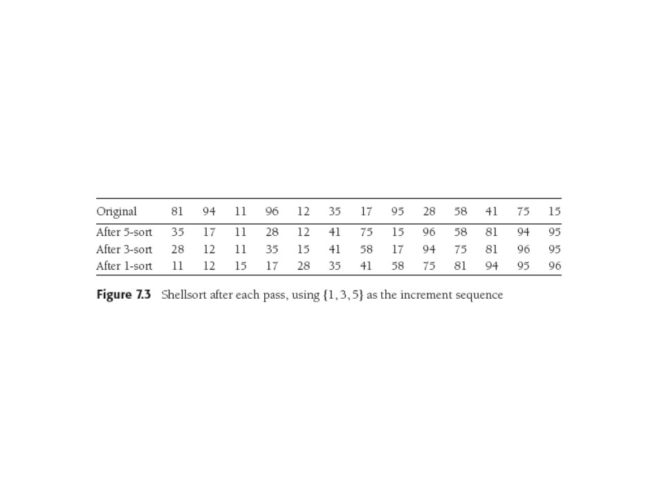
Each sorting phase orders elements that are h_k apart for one of the increments in the sequence, after which it is h_k-sorted. (We see why last increment must be 1). Why don't later sorts screw up earlier ones? (Weiss won't tell us!) Cue for you to go do some research.

Below, note that Weiss writes an increment sequence {1,3,5} despite the fact that that's increasing and 1 is first, not last. So he interprets it backwards.

Note that after the first phase, items 1, 6, 11 are sorted w.r.t each other, as are 2, 7, 12, etc. (Figure could be improved!). We're really doing insertion sort on subarrays. Note that a larger increment swaps more distant pairs (heh heh).

Shellsort worst-case Analysis

Weiss 7.4.1

In general, not easy (darned increments). Average case is open research question. Weiss shows worst-case bound for two particular increment sequences, proving worst-case running time using Shell's recommended increments is Θ(N²).

Shell's increments were {1,2,4,8,...} (in Weiss's notation). They are sub-optimal with O(N²) worst case. Whole proof is 2/3 of a page and we see a bad case:

The crux of the worst-case proof is:

• a pass with increment h_k is h_k insertion sorts of about N/ h_k elements.
• insertion is quadratic, so pass cost is
  O( h_k (N/h_k)²).
• so over all passes, cost is _i=1Σ^t (N²/h_i) =
  O(N² _i=1Σ^t (1/h_i)).
• That sum of inverse Shell increments is a geometric series with ratio 2, clearly summing to 2 with an infinite number of increments, so O(N²).

You might imagine you'd want the increments to be relatively prime so they don't step on each other. That's Shell's increments' problem, in fact. Hibbard's increments are numerically close to Shell's but have better theoretical and practical performance: 1, 3, 7, ...2^k - 1. In fact Weiss proves that with these increments Shellsort is Θ(N^3/2). Proof is not hard but non-trivial, wind up with geometric series to sum.

Of course this is not the end of the story. Sedgewick achieves bounds of O(N^4/3), with O(N^7/6) a conjectured average running time. Good sequence is:
[ 1 5 19 41 109 ...] ,whose terms are either
9*4ⁱ - 9*2ⁱ +1
or 4ⁱ-3*2ⁱ + 1 (currently "best", but who knows?)

Shellsort practical up to N ≅ 10,000, and its simplicity makes it a favorite.

Heapsort

We recall we claimed heaps can sort in NlogN time, which would be the best Big-Oh performance we've seen so far.

Build the binary heap in O(N), do N deleteMins in NlogN time, which save in second array. Moderate "oops" there, since space is often a problem practically. So since heap is shrinking, after all, fill it up from the right (a newly empty slot!) with the sorted elts as it shrinks. This reverses order, but can always substitute a (max)Heap for (min)Heap, and vice. v.

Heapsort Analysis

Simply examining the code or rereading Ch 6: heap building uses < 2N comparisons, and deleteMax is never worse than 2⌊log(N-i+1)⌋, for total of 2NlogN - O(N) comparisons. Experimentations show Heapsort usually uses about all the operations in the worst case bound. Average case analysis uses an ingenious, possibly indirect, approach to prove:

Theorem 7.5 The average number of comparisons in heapsort of a random permutation of N distinct items is 2NlogN - O(Nlog log N).

The proof works by defining the cost sequence: that is 2d_i comparisons for each deleteMax that pushes the root down d_i levels. The proof needs to show there are only an exponentially small fraction (in fact (N/16)^N) of heaps that have cost smaller than
N(logN - log log N - 4). That is, very few heaps have small cost sequences. Proof is pretty simple, basically just counting.

Can also prove Heapsort always uses at least NlogN-O(N) comparisons, and there are input sequences that achieve this bound. Also, it turns out with more work the average case can be improved to 2NlogN-O(N), with no pesky log log term.

Mergesort

Mergesort PPT. Mergesort.

List Mergesort PPT. Recursive splitting of linked list.

Mergesort Analysis PPT. Telescoping Sol'n for Recurrence Relation.

Mergesort in C PPT. E.g. C code and use of pointers.

First of two elegant, divide-and-conquer, recursive sorts. O(NlogN) worst case.
Basic operation: merging two sorted lists, which is O(N), one pass thru input if output to 3rd list.

Obvious merge implementation moves pointers thru lists or along arrays, spitting out what's under one or the other and advancing it depending on the comparison. MAW-style "Movie" p. 282-4. Sorting 1-long lists is easy, so the recursive divide and conquer algorithm is easy. Code in Fig. 7.9 has some nice subtleties that save space.

Analysis yields what we've called the "quicksort recurrence", is also the best-case, and average-case, but not worst-case, of Quicksort and also of BSTs.

Analyzing Recursion

We've seen Big-Oh analysis of straight-line code, loops, if-then-elses, function calls. Now, we do recursion.

• Special case of function call
• PRINCIPLE: The work done by a program is the sum of all work done at every level throughout the calling tree (at a 'level' and below that level in function calls).
• COROLLARY: Thus it is all the work (straight-line, if, loop, case, etc.) in a level plus 'recursively' all the work in its function calls (the function call is 'free' or O(1)).
• BASIC FACT: when 'recursively' above is really recursively, the function we're analyzing calls itself, we can write recurrence equations to express the total work or time, T(N). Getting O(T(N)) is the next goal.
• BASIC MATH LUCKY BREAK: in that case, the repeating structure imposed on the tree by re-using T(n) induced on the tree yields equations we can solve. Hence solving recurrences.

Example: Mergesort Recurrence

Related to quicksort analysis, so basic and important.

T(N) = O(1) [or O(N)] + T(N/2) + T(N/2) + O(N)
That is, at any level we need to:
SPLIT: divide the problem into two half-sized sub-problems (O(1) in best case of array, O(N) for linked list)
mergesort two half-sized sub-lists (solve the two half-sized problems),
RECURSE: call mergesort on the two halves, and
MERGE: conquer by merging two half-sized merge-sorted lists into one sorted list (O(N)).

This is a basic divide and conquer strategy.

If the list to be sorted is an array, dividing can be O(1): if it's a linked list it will take O(N) (see PPTs), but O(N)+O(N) = O(N) so what follows is still correct.

We write the mergesort recurrence as
T(1) = 1 (nothing to do but a test)
T(N) = 2T(N/2) + N
(divide, recurse, conquer)
And these we can solve.

Example: Mergesort Analysis: Graphical vs Algebraic

Graphical Approach: general, visual, often trivial, but can call for some "mathematical maturity", (persistence, intuition, experience, knowledge.)

Algebraic Approach: important special cases, "turn the crank"-ish, need careful work and sometimes some ingenuity. Often the relevant equations fall out easily from the graphical appoach.

Our textbook and for the last 10 years: strictly algebraic. This year, not.

Mergesort Analysis: Graphical

0. Split can be done fast (in-place array version, O(1) split), so will be dominated by O(N) merge. So Just Ignore It! (Typical O(N) simplification)
1. Top Level: O(N) work: (1 split), merging 2*(N/2) subproblems from below.
2. 2nd Level: O(N) work: (2 splits), merging 4(N/4) subproblems.
etc.
3. So O(N) total work at each level.
4. How many levels L? L = log₂ N by familiar arguments: basically
2^L = N.
5. So O(NlogN) work.

Mergesort Analysis: Guess plus Induction

Examples in Solving Recurrences. Guessing could be blind (bad), based on unrolling or telescoping, experience, based on partial solution or diagrams...

We see the use of induction hypothesis without our normal "assume for k-1, prove for k" approach. This is more like "assume recurrence soln is O(n), see if the recurrence equation preserves that O(n)." Obvious problem is O(n) is such a weak claim: a function that is O(1) is also O(2ⁿ)!

Hence the search for upper and lower bounds. An example in the reading above uses pseudo- induction techniques to home in on a good guess for the ultimate correct solution, and prove by showing upper bound on T(N) is same as lower bound.

Note the proof of O(mergesort) by induction is also a bit funny: prove the result of telescoping by induction, then restrict N to form 2^k and derive O(n) from that...hmmm.

Mergesort Analysis: Algebraic Astronomy

See Weiss text, sections 7.6.1, 7.7.5. Also the Solving Recurrences document.

Recurrence Equations: We need these for the Graphical Method too: they look like this.

T(1) = 1
T(N) = 2T(N/2) + N

The problem is recursively solved with two N/2-sized mergesorts followed by an N-sized merge, with nothing to do for the case of size one.

Telescoping: We'll just admire briefly. If you want to master, go for it!

Divide both sides by N to get equivalent rule *

* T(N)/N = T(N/2)/(N/2) + 1

Cute, eh? Now "telescope": math technique that uses facts that L and R sides are very similar in form, so successive use of * acts as follows:

T(N/2)/(N/2) = T(N/4)/(N/4) + 1
T(N/4)/(N/4)= T(N/8)/(N/8) + 1
...
T(2)/2 = T(1/(1) + 1

Now there are logN of these telescoping equations: can only divide by 2 log₂ times. So add them up and cancel equal L and R -side terms:

T(N)/N = T(1)/1 + logN
T(N) = N +  NlogN = Θ(NlogN).

Mergesort Analysis: Algebraic Unrolling

Unrolling: A related way to solve recurrences: pretty straightforward brute-force rewriting by repeatedly substituting right hand side into left.

our main equation. Substitute N/2 into it:

Repeating this logic by substituting N/4 into main equation,

And continuing we get in general

The space cost of copying into a temporary array can be cleverly avoided by swapping array roles between the input and temporary arrays. Also can do a non-recursive mergesort.

Master Theorem

See Weiss 10.2.1, or (better) Solving Recurrences. MAW's statement is less general, and his proofs are more long-winded: SR's has easy-to-remember 1-line proofs; geometric series!

Below, a is the number of recursive calls (pieces) in the "divide", N/b is how big each "divided" piece is, and f(N) is how much work is done at each level for "conquering".

Reasoning from the tree structure (coming up next) and geometric series, it's pretty easy to see that for any recurrence of the form
T(N) = aT(N/b) + f(N)

• if a f(N/b)= k f(N) for a const k<1,
  T(N) = Θ(f(N)).
• if a f(N/b)= k f(N) for a const k>1,
  T(N) = Θ(N^log_ba).
• if a f(N/b)= f(N),
  T(N) = Θ(f(N)log_bN).
• Else this theorem is no help.

Proof of first case: If f(N) is a constant factor larger than af(N/b), then the sum of the work at each level is a decreasing geometric series, dominated by its largest (first) term f(N).

The third case is the merge (quick)sort case, and has an even easier proof since the sum is just logN terms each equal to f(N).

You can imagine memorizing this or bringing a copy to a test, but I'm thinking there's a better way...

Recurrence Trees

Repeat:

T(N) is sum of times for all nodes. Here we count the time per level O(N) and the number of levels O(logN) so total time is O(NlogN).

Recurrence Trees-- More General

Master Theorem Cases: T(n) = aT(n/b) + f(n).

                f(n)
              /       \
[T(n/b) =]   /         \ 
       f(n/b)  a times f(n/b) =af(n/b) lev 1
       /  \             /  \
                ...           =a2f(n/b2) lev 2

Recurrence Trees-- Yet More General

Randomized Quicksort: Asymmetric tree!
T(n) = T(3n/4) + T(n/4) + n

                  n                    ^ ^
               /     \                 | | 
          3n/4           n/4           | |
         /    \        /    \      cut | log4n
    9n/16    3n/16   3n/16   n/16  |   | V
     / \      / \     / \          |   |
                                ---|   |
                                |      log4/3N
                              --|      |
...                                    |
/ end                                  V

Different values in nodes, asymmetric tree... but in a complete level nodes sum to n. Ignore all nodes below last complete level, get underestimated (lower bound) of log₄ levels. Hallucinate levels all the way to "end" and get log_4/3 levels. Lower and upper bounds = nlogn, so that's our answer.

Maybe Weirder?

T(n)=√n T(√n) +n

                   n
              /    | ...\
             √n   √n ... √n    [√n times]
            / \   ...   / \

Now say the amount of work for each node is p
-- ( e.g., p = n at the root.) That means the node's p work is broken up into √p subjobs, each of size √p, so calls for exactly p work to solve. This is true at the root where
p = n. So the work in the first and second levels is the same, and by induction it's the same for all levels and is just n.

So how many levels? Consider
n = 2⁶⁴. Note logn = 64. √n is 2³², yes? We've divided the log of n by 2 to get the square root. So how many times can we divide log(n) by 2 (take the square root) until we get down to a small number (in fact, the base of the logs... we can't get to 1)? Well, log(logn) times, natch!

We're done. T(n) = nloglogn.

Check by "induction". Most base cases are O(1)...(above, our repeated radicalizing gets us down to a 'base case' of size 2).
T(n) = n (loglog n)+n [Ind. Hyp.]
T(n) = √n √n loglog(n^1/2) + n [subst]
T(n) = n log( (1/2)log n) + n [algebra]
T(n) = n log(1/2) + n log(log n) + n [algebra]
T(n) = n log(log n) -n + n
Looks OK...

Quicksort

QuickSort PPT

Very fast, people didn't believe it'd work before recursion was actually implemented in earlier programming languages like Algol and people got familiar with the concept. O(N²) worst-case performance, but that can be made exponentially unlikely. Can combine quick- and heap sorts (Ex. 7.27).

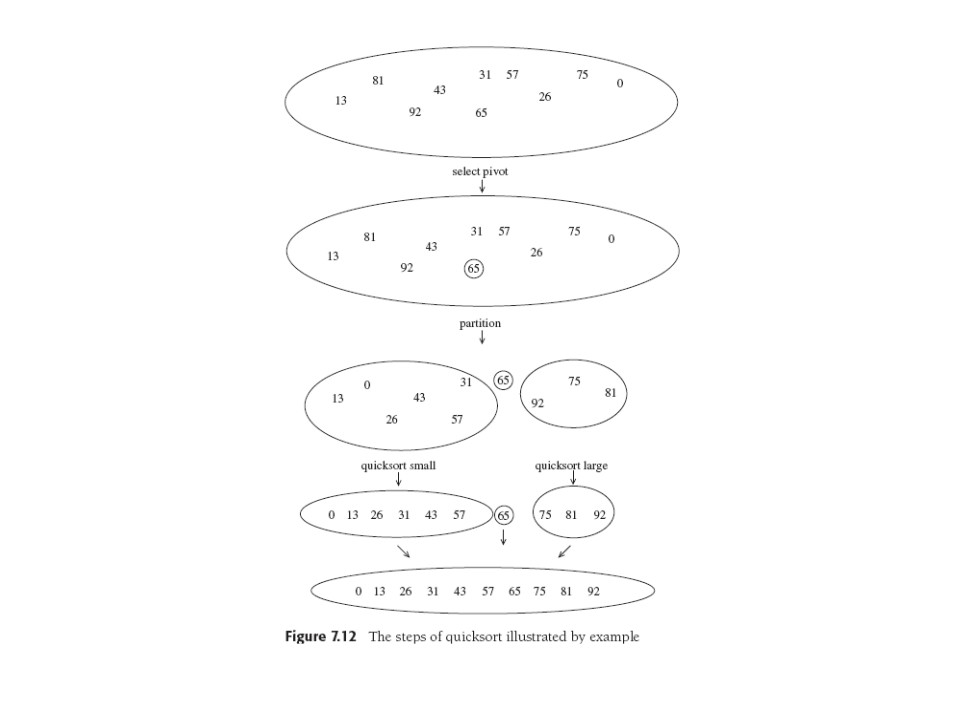
Simple idea: Chose a list pivot item, split list into "smaller", "equal", and "larger" sublists. Recursively sort 1st and 3rd list, concatenate them all, *boom*. You can see that bad choice of our special pivot item can give O(N²): send in a sorted list and pick the first item as pivot in every stage. We clearly want a pivot in the middle of the range of each list to be sorted. So "first element" is bad, "random element" not bad, and "median of first three elts" is usually good.

There are some algorithmic niddles with partitioning, with elements equal to the pivot, and other details. It's often inefficient to quicksort small arrays, so the "base case" may be to use a small-array sort like insertion. Of course Weiss gives code to look at.

Quicksort Analysis

In best case, pivot divides problem equally, get same analysis as mergesort.

Average Case: get very closely related recurrence with a sum (expressing the average) of smaller cases instead of a fixed number. Mathematics is same. Not short but not too hard: page and a half and a magic result at Eq. 7.23. Worth a look.

Oh, the Answer?: average case is O(NlogN).

Quickselect

Modified quicksort: find kth largest or smallest element. Using p-queues we saw time was O(N+klogN), so for the median it's O(NlogN). But we can sort the whole array in NlogN...can't we select faster?

Yes in the average case: the worst case of Quickselect is still O(N²) just like Quicksort's: if one of the two partition sets is always null then quickselect is not really saving a recursive call.

Its analysis (to prove average O(N) cost) is an exercise based on quicksort's. Its secret is only one recursive call, not two.

Quickselect kth smallest from set S.

1. If |S| = 1, k=1, S is answer. Or, if |S| < cutoff, sort S and return kth smallest.
2. Pick pivot v ∈ S.
3. Partition S \ {v} into S₁, S₂, as in quicksort.
4. 1. if k ≤ |S₁|, smallest elt must be in S₁, so return quickselect( S₁,k).
   2. If k = |S₁|+1, return v the pivot.
   3. Else kth smallest is in S₂ and is in fact the (k-|S₁|-1)st smallest element in S₂, so make the appropriate recursive call to quickselect.

Weiss promises us more on this topic in Chapter 10. OBoy!