Fitting Models to Data

Data Analysis

There is a cat in a box with a radioactive mouse...

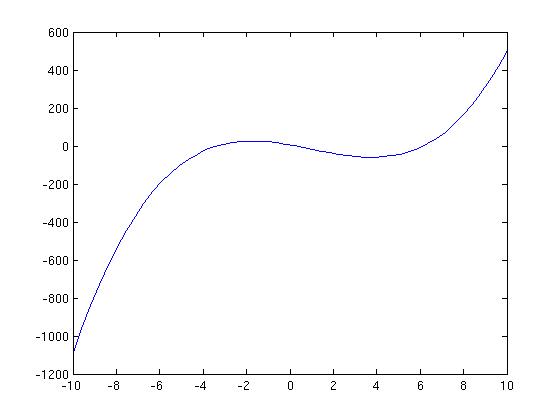
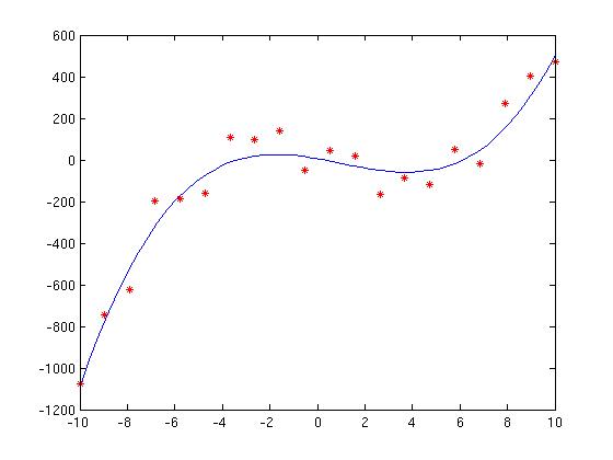
Left: A "law" or model: here a cubic polynomial. Right: Some beautiful experimental data that completely agrees with the model.

Another version of the experiment produces data corrupted by noise. Does it agree with model?

• Data analysis is all about untangling effects we are interested in from ones we are not (usually referred to as noise).
• We'll avoid traditional statistical treatment here, you'll get that soon enough elsewhere, but we'll try to give a taste of the sort of thinking and analysis involved.

Laws and Data

(RN's definition of Science:)

Science is the art of measurement.
Specifically: What can be measured, how it can be measured,
and what relationships exist between measurables.

• So science attempts to find concisely expressible relationships between quantities that can be measured.
• Many of the most useful relationships are expressed in mathematical form. If they are general and useful enough, they sometimes get the title "Law of Nature"
• The trick is how to use data we obtain from measurement to discover, explore, and use these laws.

(RN's definition of Engineering, not Dean Clark's: )

Engineering is the art of making things work.
Science is often useful for this purpose.

Noise

Noise: Any signal that interferes with the one we want.

• Systematic (Sensor bias, 60Hz hum)
• Random (shot noise, film grain, photon statistics, quantization).

Calibration is one way around "systematic noise" (reliable departure from model behavior, not worth incorporating in model itself). E.g. a clock that runs 5 minutes fast every day.

"Random noise" may be signal-dependent or signal-independent. Models employing different statistical distributions (Poisson, Gaussian, uniform...) can be used to reduce effect on measurement.

Possible Goals of Data Analysis

Assume "noisy" data.

• Describe natural phenomena with simple, elegant mathematical relations (Discover laws).
• Given a likely law in operation, discover its parameters.
• Given known law and its parameters, refine the accuracy of the parameters (e.g. the gravitational constant, the speed of light).
• Verify natural phenomena predicted by theory (in noisy data).
• Represent a relationship (of output to input, say) to predict its behavior over some input range.

Verifying a Predicted Phenomenon

A model

Measured data

Data Fitting as a System of Linear Equations

Data: vector of (x_i, y_i) pairs.
Assume process y = f(x) acts like a polynomial function of order n. We want coefficients c_i such that for every x_i, (ideally)

This is an equation in n + 1 unknowns. It has constant coefficients c_i.

For n+1 unknowns, need n+1 data points, or pairs. We fit the (x,y) pairs to the model "nth-order polynomial" by solving for the polynomial coefficients.

|1  x0 x02 ... x0n |   | c0|   | y0|
|1  x1 x12 ... x1n | . | c1| = | y1|
   ....
|1  xn xn2 ... xnn |   | cn |  | yn|

That is

y = Xc.

X is called a Vandermonde matrix. Use Gaussian Elimination to solve the system and get c_i.

The Matrix Inverse is another way to solve for c. Remember

X^-1X = I,

with I the identity matrix. So if

y = Xc, then X^-1y = c.

In fact the inverse is easily calculated during Gaussian elimation, but that need not concern us now.

Using More Data: Least Squares

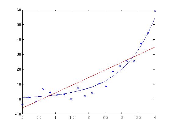
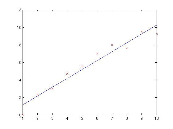
Usually, we have more data than coefficients, and it's noisy. A fit like the line below is often called a regression and the differences (vertical distances) between the data points and the line (generally function) are called residuals.

This derivation --- Derivation of Pseudoinverse --- leads to a cute result: using a matrix called the pseudo-inverse instead of the inverse gives us a solution to an overdetermined set of equations that minimizes the sum of squared residuals.

[(X^TX)^-1X^T]y = c.

Magic! Use the pseudoinverse of a non-square Vandermonde matrix and we get the least-squares solution.

If we multiply both sides of the equation on the left by X^TX we get

X^Ty = X^TXc.

This formula is in the form Ac = y' with A and y' known. This we can solve using (you guessed it) Gaussian Reduction! For technical reasons the matrix inverse can have numerical inaccuracies, so this is a better approach.

You can use your own Gaussian Elimination routines for least-squared model-fitting, and we recommend you try that (mention in your writeup if you do).

If we have a system Ax = b, with A and b known, Matlab has a shorthand x = A \ b for "solve this system for x". Note the "backslash" character used to indicate "divides into". This form should be used instead of the form x = inv(A) * b. In fact if you try the latter matlab will sometimes tell you to change it.

Goodness of Fit

Same data, different models. (Linear and Exponential). But what about quadratic or cubic? How do we decide which model to use?

One idea: use simple statistics about the residuals.

• The residuals represent the distance from the model. Their average magnitude, or the square root of sum of their squares would give a notion of "average distance" from the model curve.
• If model A is much closer to the data in this sense than model B, and we have no other reason for preference one way or the other, then model A would seem to make more sense.
• In statistics, the value related to the sum of squares is the variance. In the model-fitting case, it turns out that the best estimate for this variance must incorporate the fact that we essentially already "used up" some of our data in obtaining the model parameters.
• Specifically, if we solved for p parameters, we reduce the number of samples by p when we divide the sum of squares to obtain the variance &sigma².

  &sigma² = [1/(N-p)] &sum (y_i - model(x_i))²

• Clearly the number of samples, N must be larger than the number of model parameters p. In the case of an nth-degree polynomial, p is n + 1.

MORE: Degrees of Freedom

Consult your statistics or higher-level engineering profs for this.

Statistics, are numbers summarizing facts about a population. We need to count honestly the evidence used to calculate a statistic The degrees of freedom is just a fancy name for the count of independent pieces of information (numbers) we use.

Some statistics have a close analog to physical quantities.

One thing statistics does is estimate properties of large populations (like voters) based on samples (like polls). We want to estimate the "actual" mean and variance of some population from a number N of samples.

Our problem: Setting

Variance = &Sigma (X_i -&mu)² / N

(where &mu is the mean) turns out to underestimate the true variance (it's biased).

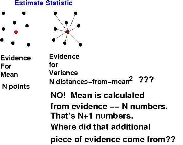
To compute the variance we need the mean. Since the mean is a linear combination of the existing evidence, we have only N-1 independent pieces of evidence (numbers) in addition.

Each independent number or parameter represents a degree of freedom, and the total number of those is bounded by the initial sample size N.

The mean depends on the N evidence points: changing one changes the mean. They're not independent. Thus using the mean "for free" is like polling someone twice: we're double-counting a DOF.

Polynomial Fits

A polynomial model (or any other model with parameters) is analogous to a "mean" that consumes several degrees of freedom - one for each parameter, instead of just one.

Specifically, suppose we use the N data points to determine an n^th- degree polynomial model

P(x) = a₀x⁰ +a₁x¹+... +a_nxⁿ = 0

with n+1 coefficients. These depend on the N data points!. To use the coefficients in addition to all the data points to calculate variances is double-dipping. We must subtract off the DOFs of those dependent numbers, hence

&sigma ² = &Sigma(Data(x_i) - P(x_i))²   /   (N - (n+1))

with &sigma the standard error of residuals, directly corresponding to the "standard deviation" we already know about.

Guessing the Form of a Model

Best case is knowing a theory of where the data came from: what law should be explaining it (mostly, or apart from noise...)?

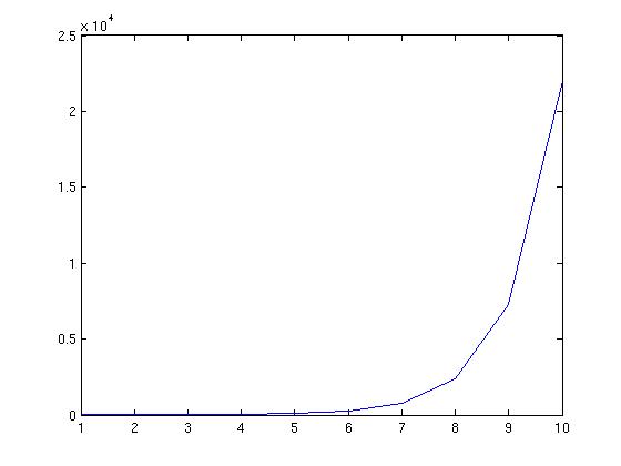
Getting the wrong law can be quite BAD. Makes extrapolation beyond known data almost certainly very wrong. E.g., the exponential of any number >1 sooner or later grows faster than any polynomial.

Worst case, Plot the data and eyeball a curve through it.

Well, maybe an even worse case (but often done), fit increasing-order polynomial models until you find a favorite (lowest order that fits well enough). Overfitting not wanted.

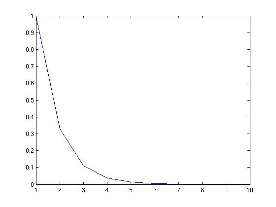
Exponential Functions

Exponential decay or explosion:

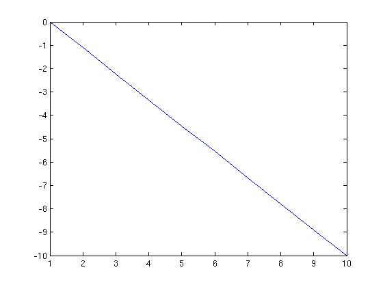
Trick: if

y(t) = e^kt,

then if we take the log of the right hand side,

y(t) = kt,

is a line!!

Expect exponential function: take log of data and see if that lies in a straight line.

Power Law Functions

Power laws are common:

• Inverse functions like Boyle's law:

  V = k/P, V = kP ^-1

• Inverse-squared Newton's law of Gravity:

  F(r) = (Gm₁m₂)/ r² = (Gm₁m₂)r^-2,

• Flow in a pipe under some conditions is &prop D⁴ (Pouseuille's Law).

y(t) = k t^m.

to obtain

log(y(t)) = m log(t) + log k.

Again a line, this time in log(t).

Expect power law? Take log of independent (say distance, time) and dependent variable (data readings), and see if they lie in a straight line.

Interpolation Polynomial

What if we have no clue of law, or desired law (say "linear") is modified by serious "systematic noise" phenomena or another law we don't fully understand (or care about).

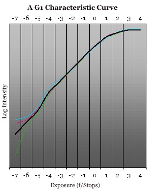
Process of calibration is common, practical example: want to estimate behavior of some instrument over some operating range, often so we can reliably interpolate and interpret its output for inputs in between the ones we used in the calibration process.

We do exactly the same as before: over the range we are interested in, pick or find an appropriate model form (a polynomial is common) and fit it to the data.

It should be reasonably good between the limits of our data (interpolation) even if the asymptotic form is wrong, and extrapolation wildly inaccurate.

Robust Techniques

Beware outliers in squared-error situations!

With sufficient care, one can iteratively remove 'outliers' from the data to obtain a better fit.

BUT... beware the ethics panel!

Central Limit Theorem

"Random" noise may be characterized by different statistical distributions (Poisson, Gaussian, uniform, ..., unknown, ...).
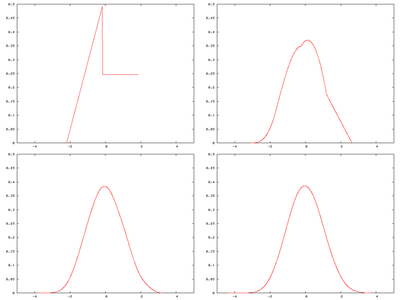
The Central Limit Theorem can justify the common use of the Gaussian, which is also very mathematically convenient.

The sum (or mean) of a large number of probability density functions of bounded mean and variance is approximately Gaussian.

(Image from Wikipedia)

1 Die Val:    1 2 3 4 5 6
Ways to Get:  1 1 1 1 1 1


Sum 2 Dice:   2 3 4 5 6 7 8 9 10 11 12
Ways to Get:  1 2 3 4 5 6 5 4  3  2  1

N₂(s) = &Sigma _x N₁(x) &sdot N₁(s - x).

N₂(s) = &int _x N₁(x) &sdot N₁(s - x) dx. Auto-convolution!