Newton-Raphson and Secant Methods

1. Newton's Method

If we only have the function defined at discrete points (say it's a vector of experimental readings, or the output of Matlab's differential equation solver, for instance), that brings in the issue of interpolation, an important numerical technique we'll ignore for now.

You may have seen this root-finding method, also called the Newton-Raphson method, in calculus classes. It is a simple and obvious approach, and is an example of the common engineering trick of approximating an arbitrary function with a "first-order" function -- in two dimensions, a straight line. Later in life, you'll expand functions into an infinite series (e.g. the Taylor series), and pitch out all but a few larger, "leading" terms to approximate the function close to a given point.

As usual, Wikipedia has a very nice article (with a movie), on Newton's method. For the mathematically inclined there's a proof of the method's quadratic convergence time: roughly, the number of correct digits doubles at every step. (BTW, the proof uses a Taylor series.)

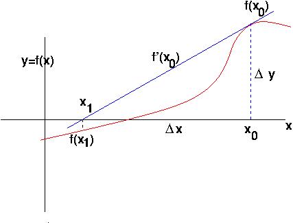
The Idea:

1. Guess an x₀ close to the root of interest.
2. Start Iteration: Approximate the function at that point by a straight line. The obvious choice is the line tangent to (in the direction of) the function's graph at that point.
3. Notice that the slope of the required tangent is the derivative of the function, so the line we want has that slope and goes through the point (x₀, f(x₀)) .
4. This tangent line goes through the x-axis at a point x₁, which is easy to calculate and which we bet is nearer to the root than x₀ is.
5. Compute x₁ and f(x₁), and we're ready to go to Start Iteration and repeat the process until for some x_i, we find a f(x_i) close enough to zero for our purposes.

Considered as an algorithm, this method is clearly a while -loop; it runs until a small-error condition is met.

The Math:

Say the tangent to the function at x = x₀ intersects the x-axis at x₁. The slope of that tangent is Δy/ Δx = f'(x₀) (where f' is the derivative of f), and Δy = f(x₀). Thus f(x₀)/(x₀ - x₁) =f'(x₀), and so x₁ = x₀ - f(x₀)/f'(x₀) . We know everything on the RHS and the LHS is what we need to continue.

Repeat until done: Generally,
(Eq. 1) x_i+1 = x_i - f(x_i)/f'(x_i).

Example: The function y = f(x) = .6x⁴ -7.533333 x³ + 29.9 x² -37.966667 x +5 looks like this:

We can see there is a root near 4.4, for instance.

f's derivative function is easy to write given f's coefficients.

3 iterations of the method starting at x₀ = 3.8, and stopping when f(x) ≤ 0.001, yields a root at x = 4.39709833506137 with error of 3.55426928955183e-06. The actual root is x= 4.39709878259766

CB's function [my_root, err] = newton(x0, maxerr) is 11 statements long, including 2 to count and print iterations and 2 to assign a global array of polynomial coeffficients. the functions function y = f(x) and der = f_der(x) are four statements, including function, global, end, and one line that actually does some work.

Extensions and Issues: There are lots of extensions, and various tweaks to the method (use higher-order approximation functions, say). The method extends to functions of several variables (i.e. higher-dimensional problems). In that case it uses the Jacobian matrix you may see in vector calculus, and also the generalized matrix inverse you'll definitely see in the Data-Fitting segment later in 160.

Clearly there are potential problems. The process may actually diverge, not converge. Starting too far from the desired root may diverge or find some other root. See a more in-depth treatment (like Wikipedia, say) for more consumer-protection warnings. To detect such problems and gracefully abort, One could watch that the error does not keep increasing for too long, or count iterations and bail out after too many, etc.

Secant Method

Here's Wikipedia: Secant method.

The Idea:

1. Pick two initial values of x, close to the desired root. Call them x₀, x₁. Evaluate y₀ = f(x₀) and y₁ = f(x₁).
2. As with the tangent line in Newton's method, produce the (secant) line through (x₀, y₀) and (x₁, y₁), and compute where it crosses the x-axis, and call that point x₂. Get y₂ =f(x₂).
3. Bootstrap along: replace (x₀, y₀), (x₁, y₁) with (x₁, y₁), (x₂, y₂) and repeat.
4. Keep this process up: derive (x_i, y_i) from (x_i-1, y_i-1) and (x_i-2, y_i-2) until y_i meets the error criterion.

The Math: Easy to formulate given we've done Newton's method. Starting with Newton (Eq. 1), use the "finite-difference" approximation:
f'(x_i) ≈ Δy/Δx = (f(x_i) - f(x_i-1)) /(x_i - x_i-1).
Thus for the secant method we need two initial x points, which should be close to the desired root.

Generally,
(Eq. 2) x_i+1 = x_i - f(x_i) [( x_i - x_i-1) / ( f(x_i) - f(x_i-1))].

Example: For the same problem as above, a reasonable function prototype is
function [my_root, err] = secant(lastx,x, maxerr). Initializing at x₀ = 3.8, x₁ = 3.9, CB gets root 4.39716813662186, with error -0.000550801803422374, also in 3 iterations. The programs are all the same size as in newton.

Extensions and Issues: The most popular extension in one dimension is the method of false position, (q.v.) There is also an extension to higher-dimensional functions.

Same non-convergence issues and answers as Newton, only risk is greater with the approximation.

The convergence rate is, stunningly enough, the Golden Ratio , which turns up all sorts of delightfully unexpected places, not just Greek sculpture, Renaissance art, Fibonacci series, etc. Thus it is about 1.6, slower than Newton but still better than linear. Indeed, it may run faster since it doesn't need to evaluate the derivative at every step.